Attrasoft ImageFinder

9.   NeuralNet Filters
9.1    Test-Driving the Logo Matching Problem
9.2   NeuralNet Filter Overview
9.3   Training
9.4   N:N Matching
9.5   1:N Matching
9.6   Summary

9.   NeuralNet Filters
The ImageFinder recognizes images in two phases:

Feature Space Matching

Input Space Matching

The purpose of Feature Recognition is to eliminate unmatched images. This Feature Recognition sub-layer has two filters:
BioFilter; and
NeuralFilter.

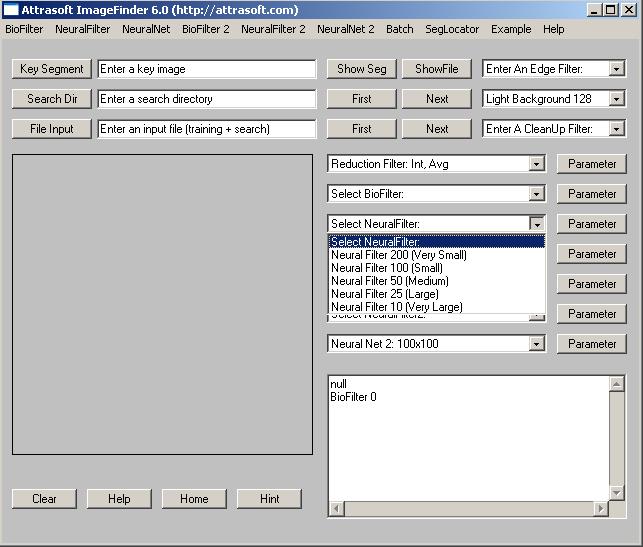
Figure 9.1 Selecting NeuralNet Filter.
The main image recognition uses the NeuralNet Filter. This chapter will demonstrate how the NeuralNet or ABM Filter works using a Logo-Matching example. The output file of the Neural Filter will be the input file of the NeuralNet Filter.
Throughout this chapter, two filters will be used: the Neural Filter works in the Feature Space Matching and the NeuralNet filter works in the Input Space Matching (Pixel Space).
Input Mode
The images are entered into the ImageFinder in two ways:

Search-Directory

Search-File

Where:

Search-Directory is a folder containing the images to be searched;

Search-File is a file listing the images to be searched.

Matching Mode
The matching can be 1:N or N : N.

1:N Matching compares one key image with the images in a search-directory or search-file; the key image is specified in the �Key Segment� textbox or selected by the �Key Segment� button.

N: N Matching compares each image, specified in the search-directory or search-file, with every image in the search-directory or search-file. N: N Matching is further divided into N: N Matching and N : (N-1)/2 Matching.

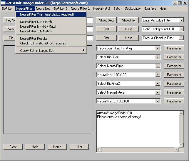
Figure 9.2 NeuralNet Menu.
In the last chapter, we have seen that for scanner images, the BioFilter will eliminate about 80% of the unmatched images and the Neural Filter will eliminate an additional 19%, leaving only about 1% of the unmatched images. In this chapter, we will use camera images. Camera images have more degrees of freedom with distances and directions, therefore, they are hard to recognize. The Feature Space Recognition alone will not be enough. The NeuralFilter will eliminate 95%, leaving only about 5% of the unmatched images for the NeuralNet Filter.
Throughout this chapter, we will use a Logo Recognition example. There are 489 images in this example, representing about 30 different Logos. They are located in the directory �.\neuralnetex1�, where �.\� is the ImageFinder software location.
9.1     Test-Driving the Logo Matching Problem
We will go through the following steps in this section:

Feature Space Recognition

Input Space Recognition

For Feature Space Recognition, the steps are the same as the last chapter:

Initialization

Converting Images to Records

Training

Template Matching

Results

For the Input Space Recognition, the steps are:

Initialization

Pixel Matching

Results

Initialization sets the ImageFinder parameters. In the Feature Space Recognition, the ImageFinder then maps an image into a record in a feature space and does a matching with the records. In the Input Space Matching, the ImageFinder works with the pixels directly.

Figure 9.3 An image in �.\neuralnetex1�.
There are 489 images in this example; they are located at the directory �.\neuralnetex1�, where �.\� is the ImageFinder software location. In the following, we will combine the initialization of the NeuralNet Filter and Neural Filter together.

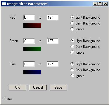
Figure 9.4 Threshold Filter Parameter.

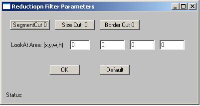
Figure 9.5 Reduction Filter Parameter.

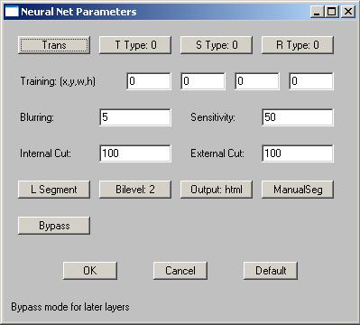
Figure 9.6 Neural Net Filter Parameter.
Summary of Parameters

1. Edge: Sobel 2
2. Threshold:
Average Filter
155 255 Dark Background
155 255 Dark Background
155 255 Dark Background
3. Clean Up: Small
4. Reduction: Default
Parameters:
Border Cut = 9

5. BioFilter: 6
6. NeuralNet Filter: 200 (Very Small)
Parameters:
Opening = very small
Threshold = 1200

7. Neural Net: 100x100
Parameters:
Blurring = 32
Sensitivity = 80
Internal Cut = 50
External Cut = 82000
Output = text
Segment type = �AutoSeg 10�

Initialization of Neural Filter

The first drop down list is �Edge Filter�; select �Sobel 2�(Second choice).

The second drop down list is �Threshold Filter�; select �Average Filter� and set it to (See Figure xxx):

155 255 Dark Background
155 255 Dark Background
155 255 Dark Background

The third drop is �CleanUp Filter; select �Small� (first choice).

The fourth drop down list is �Reduction Filter�; use the default setting. Click the Parameter button next to it and set Border Cut to 9 (See Figure xxx). We will explain the Border Cut parameter later. To set the parameter, keep clicking the button.

The fifth drop down list is �BioFilter�; use the �BioFilter 6� setting.

The sixth drop down list is �NeuralFilter�; select the �NeuralFilter 200 (Very Small)� setting.

To set the Neural Filter parameter, click the �Parameter� button next to the NeuralFilter and set:

�Neural-Filter Scale� = 0.
�Neural-Filter Opening� = Very Small
�Neural-Filter Threshold� = 1200
Initialization of NeuralNet Filter

The seventh drop down list is �NeuralNet Filter�; use the default setting.

To set the NeuralNet Filter parameter, click the �Parameter� button next to the NeuralNet Filter and set (Figure 9.6):

Blurring = 32
Sensitivity = 80
Internal Cut = 50
External Cut = 82000
Output = text
Segment type = �AutoSeg 10�

Again, we will explain these parameters later.
Converting Images to Records
We have done similar steps in the last two chapters:

Click �Search Dir� button to specify the search-directory, which contains the search images. After the �Open Dialog� dialog box comes up, go to �.\neuralnetex1� and select any file in the folder. This will specify the input directory.

Click menu item �BioFilter/Scan Images - Directory Input� to convert images to records. You should see the ImageFinder scan through the images at this point. The results will be in a1.txt.

Neural Filter Training
Neural Filter training requires two files, a1.txt and match.txt. This file has been prepared for you in advance.

Go to the ImageFinder folder, (the default folder is C:\program files\Attrasoft\ImageFinder 6.0\�), and open the file, neuralnetex1_match.txt. Save it to match.txt (overwrite the existing file). Now the training file is prepared.

Click �NeuralFilter\Train (match.txt required)�.

Template Matching

Click menu item �NeuralFilter/Query Set + Target Set/a1 + a1 ==> b1� button to do the matching.

The results are in a file b1.txt, which will be opened at this time. Go to the last line, you will see:

Total Number of Matches = 13,575
The result file contains 489 blocks. The number of blocks is the same as the number of images in the search directory, i.e. each image has a block. Line 1 in each block is input and the rest of the lines are output.

Input Space Matching

The b1.txt can be used as input for the NeuralNet Filter, however, 13575 matchings will take a long time. Instead, we will use just the first Logo, rather than all 30 Logos. The Recognition Accuracy is comparable for all 30 Logos.
Cut the 17 blocks from b1.txt and put it into a file, �b1_neuralnetex1_1.txt�. This file is already prepared for you in advance. The file looks like this:
.\neuralnetex1\76e_01l.jpg
.\neuralnetex1\76e_01l.jpg
.\neuralnetex1\76e_02l.jpg
.\neuralnetex1\76e_05m.jpg
�
The Neural Net Matching Steps are:

Click the �File Input� button and select �b1_neuralnetex1_1.txt�. The ImageFinder will check each image to make sure it exists. Wait for a while until you see:

Number of blocks = 17
Block 0. Length = 84

Click menu item �NeuralNet/1:N File Search� button to do the matching.

The NeuralNet Filter will process several images per second. The file �b1_neuralnetex1_1.txt� has about 550 matches so the computation will take a few minutes. At the end of the computation, a file will be opened and the output looks like:
Training: C:/.../76e_01l.jpg
C:/.../76e_01l.jpg 344000
C:/.../76e_02l.jpg 100800
C:/.../76e_06l.jpg 112640
C:/.../76e_12l.jpg 93760
C:/.../76e_18l.jpg 84032
C:/.../spu_03l.jpg 83008
--------------------------
Training: C:/.../76e_02l.jpg
C:/.../76e_01l.jpg 102272
C:/.../76e_02l.jpg 130560
C:/.../76e_07l.jpg 95104
C:/.../76e_08l.jpg 82432
C:/.../76e_13l.jpg 89408
C:/.../76e_15l.jpg 96448
C:/.../net_03s.jpg 84352
C:/.../net_17m.jpg 84352
C:/.../war_16l.jpg 82752
--------------------------
Training: C:/.../76e_03m.jpg
C:/.../76e_03m.jpg 192000
C:/.../76e_16m.jpg 95808
C:/.../76e_17m.jpg 97600
--------------------------
Results
In the above output, �Training: C:/.../76e_01l.jpg� is the input file. This image is compared with 489 images. The Neural Filter reduces the number of comparisons from 489 to 84. The NeuralNet Filter further reduces the number of comparisons from 84 to 6:
C:/.../76e_01l.jpg 344000
C:/.../76e_02l.jpg 100800
C:/.../76e_06l.jpg 112640
C:/.../76e_12l.jpg 93760
C:/.../76e_18l.jpg 84032
C:/.../spu_03l.jpg 83008
The first one is self-matching and it does not count. Out of the rest of the 5, the highest score is 112640, which classifies the input image, 76e_01l.jpg, to category 76e_06l.jpg, which is correct.
16 out of 17 Logos are classified correctly.
The Identification Rate is 94%.
To speed up the neural computing, select a different NeuralNet Filter:
Neural Net: 50x50
Blurring = 25
Sensitivity = 70
Internal Cut = 100
External Cut = 0
Output = text
Segment type = AutoSeg 10
This time, the computation is much faster. The result is:

Training: C:/.../76e_01l.jpg
C:/.../76e_01l.jpg    770000
C:/.../76e_02l.jpg    13372
C:/.../76e_12l.jpg    12634
C:/.../76e_18l.jpg    12598
C:/.../pis_10l.jpg    11194
----------------------------------------
Training: C:/.../76e_02l.jpg
C:/.../76e_02l.jpg    130700
C:/.../76e_07l.jpg    12886
C:/.../76e_08l.jpg    12274
C:/.../76e_13l.jpg    13408
C:/.../76e_15l.jpg    13192
C:/.../cli_05m.jpg    12544
C:/.../cli_10m.jpg    12526
C:/.../kin_01m.jpg    12868
C:/.../mag_01m.jpg    12634
C:/.../net_17m.jpg    13282
----------------------------------------
Training: C:/.../76e_03m.jpg
C:/.../76e_03m.jpg    136000
C:/.../76e_17m.jpg    13318
----------------------------------------
Training: C:/.../76e_05m.jpg
C:/.../76e_03m.jpg    12220
C:/.../76e_05m.jpg    700000
C:/.../76e_17m.jpg    12238
C:/.../cli_10m.jpg    12148
C:/.../net_11l.jpg    11860
C:/.../pis_10l.jpg    11230
C:/.../pis_13l.jpg    11752
----------------------------------------
Again, 16 out of 17 Logos are classified correctly. The Identification Rate is 94%.
Now, identify the entire 489 images:

Click the �File Input� button and select �b1.txt�. The ImageFinder will check each image to make sure it exists. Wait for a while until you see:

Number of blocks = 489
Block 0. Length = 84

Click menu item �NeuralNet/1:N File Search� button to do the matching.

9.2   NeuralNet Filter Overview
The ImageFinder recognizes images in two phases:

Feature Space Matching

Input Space Matching

The Feature Space Matching will be done in several steps:

Initialization

Converting Images to Records

Training

Template Matching

Input Space Recognition Steps are:

Initialization

Pixel Matching

Results

We have discussed Feature Space Matching in the last two chapters.
Let us look at Input Space Matching:
Initialization
Initialization sets the ImageFinder parameters.
Entering Data:
The output of the Neural Filter, b1.txt, can be used as the input for the neural net matching. If this file is too large, you can split it into several pieces and match one piece at a time.
Training and Matching
NeuralNet Filter learns the first image in each block and matches it against the rest of the images in the block.

9.3   Training
Training teaches the ImageFinder what to look for. Each filter is trained differently. NeuralNet Filter learns directly from the training image, therefore, a match file will not be required.
9.4   N:N Matching
When using file input, N: N Matching compares each image in the block against every other image in the block. N: N Matching will be done only to the very first image block in the input file.
9.5   1:N Matching
Again, 1:N Matching compares the first image in a block against the rest of the images in the block. 1:N Matching can handle many 1:N Matchings at the same time. For example, in early this chapter, a single click will handle 17 comparisons.
9.6   Summary
I. Preparations
Data
Data is stored at �.\neuralnetex1�. There are 489 images.
Neural Filter Training File
1. The Training file must have the name �match.txt�;
2. Find the file, �.\neuralnetex1_match.txt�, and save it to match.txt.

II. Operation

Start the ImageFinder;

Edge Filter: select Sobel 2;

Threshold Filter: select Average Filter;

Set the Avg Filter
155 255 Dark Background
155 255 Dark Background
155 255 Dark Background

CleanUp Filter: select Small;

Reduction Filter: Default; Reduction Filter Parameter: Border Cut = 9

BioFilter: select 6; BioFilter Parameter: default;

Entering Data: click �Search Dir� and select any file in �neuralnetex1� directory;

Converting to Records: click menu item �BioFilter/Scan Images - Directory Input�;

Neural Filter Training: click �NeuralFilter\Train (match.txt required)�;

N:N Matching: click click �NeuralFilter/Query Set + Target Set/a1 + a1 ==> b1�;

Attrasoft Matches: go to the last line of b1.txt and see: �Total Number of Matches = 13575�;

Click the �File Input� button and select �b1_neuralnetex1_1.txt�; The ImageFinder will check each image to make sure it exists. Wait for a while until you see:

Number of blocks = 17
Block 0. Length = 84

Click the menu item �NeuralNet/1:N File Search� button to do the matching;

Results, 16 out of 17 are identified.

Return