Attrasoft ImageFinder
User’s Guide
1.1 What will the
ImageFinder do?
1.2 ImageFinder
GUI (Graphical User Interface)
6.1 Finding
Duplicated Documents
8.6 Load
Multiple Libraries and Additional Libraries
11.1 Set Image
Preprocessing Filter
11.5 Skip the
Empty Border by Content Percent
12.2 Set Image
Processing Filters
15.1 Document
Matching Example
16.6.8
Internal/External Weight Cut
1. Introduction
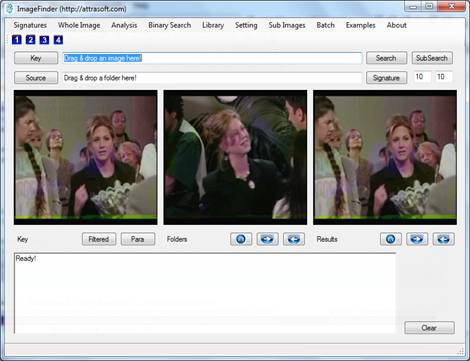
Figure 1.1 ImageFinder.
Image Recognition technology will increasingly replace human labor in the form of:
- Creating new products; or
- Improving existing products/processes to increase productivity,
which will translate into saving
man-hours, saving money, making more money with fewer resources, doing new
things, and/or shorten service turnaround time. Applications are limited only by your imagination:
Biometrics
Video - Image
Recognition
Content-Based
Advertisement
Statistics Collection (advertisement statistics, …)
Internet
Audio-Visual Search Engine
Satellite
Image Recognition (defense)
Cancer
Detection (medical)
Content-base Image Retrieval (digital library)
Space Image Recognition (space exploration)
Object
Detection (military)
Face Recognition, Fingerprints, Palm Prints (security locks & systems)
Stamp
Recognition (post office)
Trademark
Search
Real Time
Event Detection
Forensic Identifications
Etc.
1.1 What will the ImageFinder do?
The ImageFinder is image recognition software for:
- Searching a whole image;
- Searching a sub image.
1.2 ImageFinder GUI (Graphical User Interface)
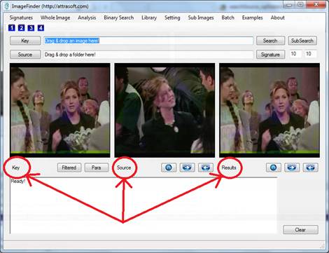
Figure 1.2. Three image Panels: Key, Source, and Results.
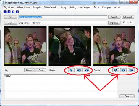
Figure 1.3 First, Next, and Previous button for a Source,
and First, Next and Previous button for
match Results.
The ImageFinder has three image panels (Figure 1.2):
·
Key Panel;
·
Source Panel; and
·
Results Panel.
Key
A key is an image or an image segment to be searched. Dragging & dropping an image into the first text box will select a key.
Source
A folder is a collection of previously stored images. Use the Home, =>, and <=buttons in Figure 1.3 to see the images in the folder. The Home button goes to the first image; the “=>” button goes to the next image; and the “<=” button goes to the previous image. All sub-folders will be included. Dragging & dropping a folder into the second text box will select a Source.
Results
Results are images that matched the “key” image. Use the Home, =>, and <= buttons in Figure 1.3 to see matched images. The Home button goes to the first image; the “=>” button goes to the next image; and the “<=” button goes to the previous image. Results are generated by a 1:1 or 1:N match.
1.3 Customized Software
The ImageFinder for
Windows has 100 open parameters for the user to adjust for their particular
image type. However, the ImageFinder itself has 3000+ internal
parameters, which the users have no access to at all. To get maximum accuracy
for a particular problem, customization will be required. If you need a
customized version of the ImageFinder, please contact gina@attrasoft.com.
Customized versions
can accommodate:
- Customized tweaking;
- Speed Optimization;
- Storage Optimization;
- Graphical User Interface Customization;
- Database interface;
- Video processing;
- New Image Preprocessing Filters;
- Customized Filters;
- Programming Library;
- Specific Symmetries or Combination of Symmetries;
- Attrasoft can implement any symmetry (or combination of symmetries) which can be described by mathematics;
- Further refinement Tuning for small image segments;
- Digital Image Database (Combine ImageFinder with Database);
- Counting objects which are NOT physically separated;
- Internet Image Search Engines;
- Web Interface;
- Other Specific Needs.
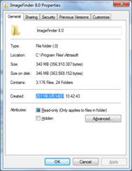
1.4 Installing the Software
To Install:
· Click “CD:\setup.exe”;
· Remove program folder Read-only attribute;
· Give program folder Read & Modify Permissions.
Detail:
· Click “CD:\setup.exe”;
· To remove the Read-only attribute, open Windows Explorer, and go to the program folder; the default folder is:
C:\Program Files\Attrasoft\ImageFinder 8.0.
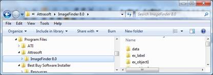
Right click the folder and select Property to get the Figure below, and uncheck the Read-only button.
· To give Read & Modify Permissions, go to the Security tab in the Figure above to get the Figure below,
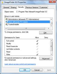
Click the “Edit” button in the Figure above to get the Figure below:
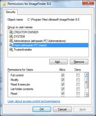
Check the Modify box and the Write box, and click the “OK” button.
To Uninstall:
· Click “CD:\setup.exe” again.
1.5 Test Installation
Open Windows Explorer and go to the program folder; the default folder is:
C:\Program Files\Attrasoft\ImageFinder 8.0\.
We will call it “.\” folder.
· Click the “1” button on the toolbar to select directory, .\test\.
· Click the “2” on the toolbar to compute the signatures.
· Click the “3” button on the toolbar to select an image, .\test\ L01008gi_r90.jpg.
· Click the “4” button on the toolbar to search.
2. ImageFinder Overview
2.1 Menus
When searching for an image, the image is converted into image signatures and the search is based on image signatures. The “Signature” menu provides menu items to compute the image signature.
“Whole Image” menu provides menu items to search a whole image sequentially.
“Analysis” menu provides menu items to compare the computer generated results with the human generated results and provide computational statistics.
“Binary Search” menu provides menu items for binary search, which is faster than sequential search, but harder to maintain.
“Library” menu provides menu items to search dynamically, i.e. search while adding, deleting, and modifying image signatures. It also has advantages over the “Whole Image” menu and the “Binary Search” menu by allowing a single loading of the search library, so the library will need not be loaded over and over again.
“Sub Image” menu provides menu items to search inside an image.
2.2 Overview of Chapters
Chapter 3 introduces Image Signatures. Features of an image are computed and a collection of features is grouped into a signature.
Chapter 4 introduces matching for whole image against whole image.
Chapter 5 introduces analysis of computational results.
Chapter 6 presents several examples: finding duplicated Document images and identifying Faces from a photo ID.
Chapter 7 introduces binary search, which is faster than sequential search, but harder to maintain.
Chapter 8, Dynamic Library, briefly describes the matching process where the Master Library is constantly updated via insertion and deletion.
Chapter 9 introduces the sub image search.
Chapter 10 introduces a few faster commands.
Chapter 11, Image Preprocessing, briefly describes the image preprocessing process required for the ImageFinder.
Chapter 12, Image Processing, briefly describes the image processing process required for the ImageFinder. You have to set three filters: Edge Filters, Threshold Filters, and Clean-Up Filters. The Threshold Filter is required; the other two filters are optional.
Chapter 13, Signature Filter, briefly describes how different image signatures can be computed.
Chapter 14,
Batch, introduces the batch command, which allows you to save your settings and
reload your settings.
Chapter 15, Training, describes the training process for the ImageFinder.
Chapter 16, Parameters, describes the open parameters in the ImageFinder.
Chapter 17,
Application Developer, introduces the procedure for developing an image
recognition application.
Chapter 18, Reference Manual lists and explains the important menu items.
3. Image Signatures
Image Matching is done through something called Image Signature. An image has a set of computed values called features. A collection of features is grouped into a signature.
Signature Menu computes signatures in the ImageFinder: the input is an image and the output is a signature.
Image matching has three types:
1:1 matching – 1 to 1 matching.
1:N matching – 1 to many matching.
N:M matching – many to many matching.
We will show how to use the image signatures in the next chapter. This chapter introduces how to compute signatures only, which will take an input image and produce a signature. This chapter will also compute image signatures for various variations of an image.
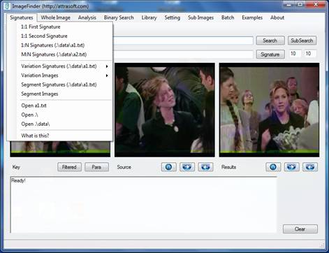
Figure 3.1 Signature Menu.
3.1 Signature Menu
Figure 3.1 shows the menu items under the Signature Menu. You can collect the signature(s) from:
- A selected key image;
- The current source image; and
- All of the images in a source folder, including all of its sub-folders.
3.2 Key Signature
To compute the signature of a key image:
- Click the “Key” button to select a key image or sample image;
- Click the “Signature/1:1 First Signature” to compute the signature.
Example. Key Signature.
- Click the “Key” button to select “.\ex_wheel\2067(1).jpg”;
- Click the “Signature/1:1 First Signature” to compute the signature.
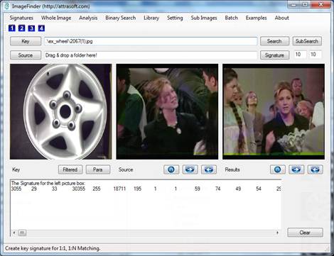
Figure 3.2 Compute
a Key Signature.
The Signature looks like:
3055 29 33 30355 255 18711 195 1 1 …
In 1:1 Matching or 1:N Matching, the signatures are computed behind the screen; you do not need to use the signature directly. The menu item, “Signature/1:1 First Signature”, shows you the mechanism behind the screen so you can see what a signature looks like.
3.3 Signature Files
In 1:N Matching, the key image will be matched against all images in a directory. In particular, the key signature will be matched against all image signatures in a directory; we call them 1-Signature and N-Signatures, respectively.
Key-Signature
The key signature is computed first, as we have shown in the last section. Then this signature will be matched against all signatures in a file, called the N-Signature file.
N-Signature File
The N-Signature file has a fixed name, “.\data\a1.txt”. Here “.\” means the folder where the ImageFinder is located and “.\data\” is the folder.
M-Signature File
In N:M Matching, the N-Signature file, a1.txt, and the M-Signature file, a2.txt, are computed first. Then each of the signatures in a1.txt will be matched against all of the signatures in a2.txt. The M-Signature files have a fixed name, “.\data\a2.txt”.
There are 2 menu items:
- Signature/1:N Signature (.\data\a1.txt)
- Signature/N:M Signature (.\data\a2.txt)
These commands compute the signatures for all images in a folder, including all of its subfolders. The only difference between the two commands is where to save the signatures.
Signature/1:N Signature (.\data\a1.txt)
Menu item, Signature/1:N Signature (.\data\a1.txt), computes the signatures for all images in a directory and saves the signatures to a1.txt, the N-Signature file.
Signature/N:M Signature (.\data\a2.txt)
Menu item, Signature/N:M Signature (.\data\a2.txt), computes the signatures for all images in a directory and saves the signatures to a2.txt, the M-Signature file.
To compute the 1:N signatures:
· Click the “Source” button to select a directory;
- Click “Signature/1:N Signature (.\data\a1.txt)” to compute the signatures in a1.txt.
Example. Compute N-Signatures:
· Click the “Source” button;
· Select folder, ./ex_wheel/, here “./” means the folder where the ImageFinder is located;
· Click “Signature/N Signature (.\data\a1.txt)” to compute image signatures;
· Click “Signature/Open a1.txt” to see the results.
3.4 Variation Signatures


Figure 3.3 A change beyond the tolerance of a single image signature.
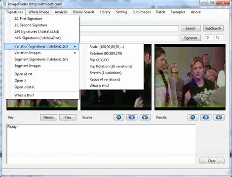
Figure 3.4 Signature/Variation Signatures Menu.
Image Matching is done through something called Image Signature. An
image has a set of computed values called features. A collection of features is
grouped into a signature. A single image signature will take care of a certain
amount of variation. To increase the variations, additional signatures will be
added, which is the purpose of the Variation Signatures menu.
An image can be changed, for example, a rotation of 90 degrees to the left. As the image is changed, the signature will change accordingly. In general, this change will not be maintained inside a signature, i.e. a small variation allowed inside a single signature will not take care of large variations like 90 degree rotations.
The “Signature/Variation Signatures” menu item (Figure 3.4) provides a list of menu items to compute signatures. The net result is that an image will have multiple image signatures.
The “Signature/Variation Image” menu item (Figure 3.5) will compute various variations of images from the key image and will deposit these images into “.\tmp\” folder. To use this menu item, you must first select a key image. This allows a user to see what the variations are.
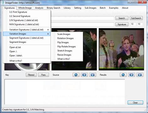
Figure 3.5 Signature/Variation Images Menu.
This menu supports the following variations:
Signatures/Variation Signatures/Scale (100, 90, 80, …)
This menu
item generates 7 image signatures:
100%, 90%,
80%, 70%, 60%, 50%, 40%.
Here 90% is
an image that has 5% border region removed.
Signatures/ Variation Signatures/Rotation (90, 180, 270)
This menu
item generates 4 image signatures:
0, 90, 180,
270.
Here 90 is
an image that has a 90 degree rotation.
Signatures/ Variation Signatures/Flip (X, Y, XY)
This menu
item generates 4 image signatures:
0, X, Y,
XY.
Here X is
an image that has flipped around x axis.
Signatures/ Variation Signatures/Flip Rotation (16
variations)
This menu
item generates 16 image signatures:
{0, 90, 180,
270} ^ {0, X, Y, XY}.
Here (90,
X) is an image that has 90 degree rotation and flipped around x axis.
Signatures/ Variation Signatures/Stretch (4 variations)
This menu
item generates 5 image signatures:
(0, 0), (120%,
100%), (80%, 100%), (100%, 120%), (100%, 80%).
Here (120%,
100%) are stretch percentages along the x and y directions.
Signatures/ Variation Signatures/Resize
This menu
item generates 5 image signatures:
100, 150,
200, 300, 400.
Here 150
increases the image size by 50% in terms of pixel counts in each direction.
To get signatures for images in a folder in your computer:
1. Select a folder;
2. Click one of the menu items in Figure 3.4.
Other variations can be added upon customization. These commands allow you to compute each individual variation. To combine all of the above variations, you will:
- Get each variation first;
- Rename the a1.txt file to avoid overwriting of the old a1.txt by a new a1.txt; and
- Use the image library to load all of the files.
We will address this in the Library chapter.
3.5 Segments
A collection of
features is grouped into a signature. One image has one signature. The signature matches whole images against whole images,
i.e. it does not look inside the image.
An image can be many logical segments. As the focus changes from a whole image to an image segment inside the image (Figure 3.6), the signature will change accordingly. In general, this change will not be maintained inside a basic signature.
The “Signature/Segment
Signatures” menu item attempts to partially address this image
segmentation problem. The menu item will look at some segments inside an image.
On average, it will look at six segments.
The “Signature/Segment Signatures” menu item (Figure 3.1) computes signatures for image segments. The net result is that an image will have multiple image signatures, one for each segment.
The “Signature/Segment Images” menu item (Figure 3.1) will compute segments from the key image and will deposit them into “.\tmp\” folder. To use this menu item, you must first select a key image. This allows a user to see what the segments are.
To get signatures for images in a folder in your computer:
1. Select a folder;
2. Click “Signature/Segment Signatures”.
Figure 3.6 Image Segmentations.
3.6 Signature Management
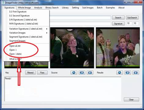
Figure 3.7 Image Signature files are managed via Windows Explorer. These commands let you quickly locate the image signature files and manage the signature files.
Once you moved from a single signature file to multiple signature files, you will need to manage the signature files via Windows Explorer. Such management activities are limited to moving files from one folder to another, and renaming files. There are three commands in Figure 3.7 to help you to locate and manage the signature files.
4. Whole Images
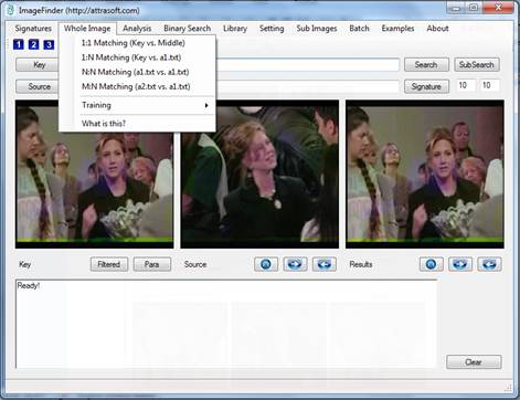
Figure 4.1 “Whole Image” Menu.
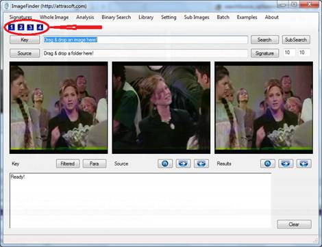
Figure 4.2 Toolbar.
To search an image, initially, you will need the following four steps:
1. Select a source (Click the “1” button in
the Toolbar, see Figure 4.2)
2. Get Library Signatures (Click the “2”
button in the Toolbar, see Figure 4.2)
3. Select a Key image (Click the “3” button
in the Toolbar, see Figure 4.2)
4. Search (Click the “4” button in the
Toolbar, see Figure 4.2)
To see the results:
1. Click the “Home” button in the Results
Panel (see Figure 4.2);
2. Click the “=>” button in the Results
Panel (see Figure 4.2).
Starting from the second search, you do not have to create an image
signature library each time; each search has only two steps:
3. Select a Key image (“3” button)
4. Search (“4” button)
3. Select a Key image (“3” button)
4. Search (“4” button)
…
This 4-step process is designed for simplicity, which will apply to
only small numbers of images. Each time you make a search, the a1.txt file is
loaded. To search a large amount of images, loading a1.txt each time will slow
down the process; so you will need to use the Library. The Library matching
adds two more steps.
4.1 Learn by Example
Data used in this example (20 images) is in folder:
.\test\
The example will take four clicks:
1.
Click the “1” button in the Toolbar,
and select folder, “.\test\”; see Figure 4.3.
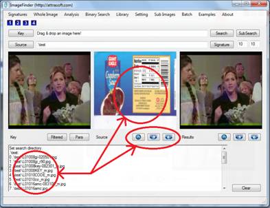
Figure 4.3 Step 1, selecting a folder. After selecting a folder, the
first image will be displayed in the Source Panel. The list of image files will
be displayed in the text window. The “Home” button goes to the first image; the
“=>” button goes to the next image; and the “<=” button goes to the previous image. All sub-folders
will be included.
2.
Click the “2” button in the Toolbar
to convert images into signatures; this step will take a minute; see Figure 4.4.
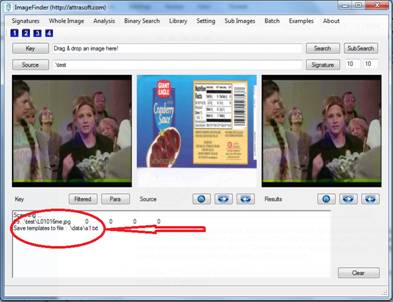
Figure 4.4 Step 2, converting images to signatures. This step will take a minute. This step will end with a message, “Save …”.
3.
Click the “3” Button in the Toolbar
and select any image, for example “.\test\L01008key-082301_m.jpg”; see Figure 4.5.
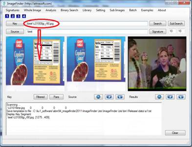
Figure 4.5 Step 3, selecting a key. After selecting a key image, the image will be displayed in the Key Panel.
4.
Click the “4” button in the Toolbar
to search; see Figure 4.6.
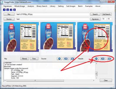
Figure 4.6
Search the selected folder. Images
that matched the “key” image will be displayed in the Results Panel. Use the
Home, Next, and Previous buttons to see matched images. The “Home” button goes
to the first image; the “=>” button goes to the next image; and the “<=” button goes to the previous image.
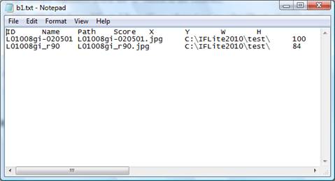
Figure 4.7 Text Output.
Figure 4.7 shows the text output. Figure 4.8 shows the visual output. To see the first matched image, click the “Home” button in the Results Panel (see Figure 4.8).
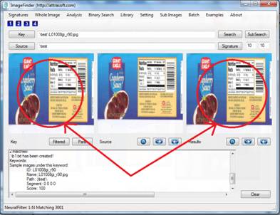
Figure 4.8 The “key” image and matched images are
displayed side-by-side.
4.2 1: N Matching
1. Select a Source (“1” button)
An image is converted into an image signature.
A set of image signatures forms a library. This step selects an image folder
that has images you want to search through. This step is implemented by:
·
Clicking
the “1” button in the Toolbar, or
·
Clicking
the “Source” button, or
·
Dragging
and dropping a folder into the second textbox.
The images in the selected folder will be
displayed in the second picture box (Source Panel).
2. Get Image Signatures (“2” button)
This step converts all images in the selected
folder into signatures and saves them to a file. This step will take some time;
after the conversion is done, a message comes out in the text window below the
picture boxes. It will say the data is saved to a file.
The last chapter computes image signatures;
in this chapter, we will use only one menu item, “Signature\N-Signatures”,
which is also the “2” button in the Toolbar.
It will take 0.1 to 1 second to convert one
image into one image signature; so if you have many images, this step can take
hours. Once a signature library for a folder is computed, you can use it over
and over again unless you later add new images to this folder, OR until you
want to search a different folder. This step is implemented by clicking:
·
“2”
button in the Toolbar, or
·
“Signature”
button.
3. Select Key (“3” button)
A key is an image you are looking for from a
folder. The key image (for example, c:\abc\def\ghi.jpg) will be entered into
the ImageFinder.
This step selects a key image by:
·
Clicking
the “3”
button, or
·
Clicking
the “Key” button, or
·
Dragging
and dropping an image into the first textbox.
The selected key image will
be displayed in the first picture box.
4. Search (“4” button)
The image will first be converted into a
signature; then it will be matched against a library of signatures. This step is implemented by clicking:
·
“Whole
Image/1:N Search” menu item, or
·
“4”
button, or
·
“Search”
button.
To see the results:
1. Click the 2nd “Home” button;
2. Click the 2nd “=>” button.
4.3 N:M Matching
To search for multiple images in a
folder, you will need N:M matching. The process is:
1. Select a folder;
2. Get Library Signatures, a1.txt;
3. Select a folder;
4. Get Library Signatures, a2.txt;
5. Match a1.txt with a2.txt.
Here, each image in a1.txt will
match against all signatures in a2.txt. The results will be given in
.\data\b1.txt. To implement this
process:
1. Click the “1” button in the
Toolbar;
2. Click the “2” button in the
Toolbar;
3. Click the “1” button in the Toolbar
again;
4. Click “Signature/N:M Signature”;
5. Click the "Whole Image/N:M
Matching (a1.txt vs. a2.txt)" menu item.
There will be many examples for N:M
matching later.
5. Results & Analysis
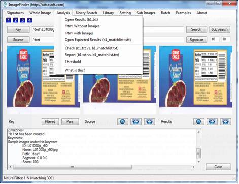
Figure 5.1 Analysis Menu.
In this chapter, we will use a simple example, Wheel Rim Identification, to give a quantitative description of the search results. The quantitative description is given by three variables. The variables are obtained by comparing the computer generated answers and human answers. The analysis is generally done for N:M matching. The Analysis Menu is given in Figure 5.1.
Human Generated Answers
The human generated results are in a fixed file, .\data\b1_matchlist.txt. This file contains all of the expected correct results. This file follows a certain format. You will need to manage the human generated results yourself. For example, you will prepare these files:
.\data\b1_matchlist_prob1.txt
.\data\b1_matchlist_prob2.txt
.\data\b1_matchlist_prob3.txt
…
For a particular problem, you will use Windows Explorer to overwrite .\data\b1_matchlist.txt by a file, say .\data\b1_matchlist_prob1.txt.
Computer Generated Answers
The computer generated results are in a fixed file, .\data\b1.txt.
To analyze a problem, the “Analysis” Menu compares the two files, .\data\b1.txt and .\data\b1_matchlist.txt and reports the results.
5.1 Wheel Rim Example
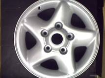
Figure 5.2 A Newly Captured Image.
The problem is: assuming we have a newly captured image in Figure 5.2, let us match it against the existing master library and see if there is a match. There are 100 images in 25 quadruplets. The data is stored at “.\ex_wheel\” folder.
In general, a product needs to be identified for the following reasons:
- Replacement of parts;
- Storage of parts in correct place;
- Check before delivery;
- Check after receiving a delivery;
- …
5.2 N:N Matching
N:N matching process is:
Signatures
- Click the “Source” button and select“.\ex_wheel” director. This will specify the input directory.
- Click the Source “>” button a few times to see the images;
- Click menu item “Signature/1:N Signature (.\data\a1.txt)” to get the signatures in a1.txt file.
N:N Matching
- Click menu item “Whole Image/N:N Matching (a1.txt vs. a1.txt)” to complete a N:N Match.
Results
The results are in a file, b1.txt, which will be opened at this time:
C:\...\2067(1).jpg
C:\...\2067(1).jpg
100
C:\...\2067(2).jpg
84
C:\...\2067(3).jpg
84
C:\...\2067(4).jpg
84
C:\...\2071(1).jpg
81
…
Total Number of Matches = 1264
The last line,
1264, indicates the number of matches in this file.
5.3 Three Output Files
A matching will produce three output files:
- b1.txt;
- b1.htm; and
- b1.html.
The text file, b1.txt, will be opened at the end of each run. This file can also be reopened via clicking “Analysis/Open Results (b1.txt)”. The two other files can be opened by clicking “Analysis/Open b1.htm” and “Analysis/Open b1.html”, respectively.
The first result file is a text file. In each block, the first line is the input and the rest of the lines are output:
Key
Match 1
Match 1 score
Match 2
Match 2 score
…
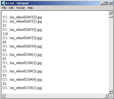
Figure 5.3 Click “Analysis/Open results (b1.txt)” to
open result file, 1 of 3.
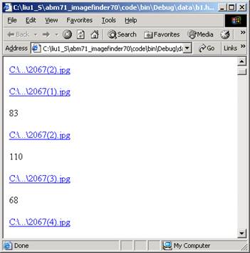
Figure 5.4 Click “Analysis/Open b1.htm” to open result
file, 2 of 3.
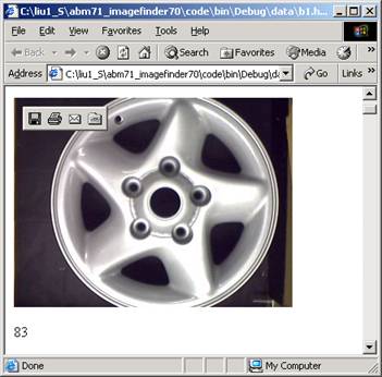
Figure 5.5 Click “Analysis/Open b1.html” to open result
file, 3 of 3.
The second result file is a html file. In each block, the first line is the input and the rest of the lines are output:
Key
Match 1
Match 1 score
Match 2
Match 2 score
Each of these lines is a link to the original images.
The third result file is a html file. In each block, the first line is the input and the rest of the lines are output:
Key
Match 1
Picture 1
Match 1 score
Match 2
Picture 2
Match 2 score
This result file displays all of the matched images.
5.4 Checking the Results
You
can find out the identification rates of your matching by a few clicks. You
must prepare a human generated result file, b1_matchlist.txt, which states who
in b1.txt should match with whom.
An example of b1_matchlist.txt is:
400
101 2067(1) 2067(1)
102 2067(2) 2067(2)
103 2067(3) 2067(3)
104 2067(4) 2067(4)
105 2067(1) 2067(4)
106 2067(2) 2067(1)
107 2067(3) 2067(2)
108 2067(4) 2067(3)
…
Line 1 is the number of matches in this file. In our example, there are 25 quadruplets, so each image should match with 4 other images, giving a total of 100 * 4 = 400 positive matches. The format is b1_matchlist.txt is:
Number, tab, filename, tab, filename.
Note:
- You MUST have a tab between the three columns;
- The file names do not contain “.jpg”.
There are two common errors:
(1) The Tab is replaced by a space;
(2) The number of rows is less than the first number in the file.
To
continue our recognition example, we must prepare the b1_matchlist.txt file
now. This file is already prepared for you and we will simply open it and save
it to b1_matchlist.txt (overwrite the existing file). The steps are:
- Open “./data/b1_matchlist_ex_wheel.txt. Save it to b1_matchlist.txt (overwrite the existing file). Now this file is prepared.
- Click “Analysis/Check (b1.txt vs. b1_matchlist.txt required)” to check the results.
You
will see something like the following in the text window:
Blocks = 101
…
Total Matches = 378
The message indicates b1.txt has 101 blocks: the 100 image blocks plus the last line indicating the total number of matches retrieved. The message “Total Matches = 378” indicates that 378 matches in b1.txt agree with those in b1_matchlist.txt. Matching results, 378 out of 400, can be improved by training.
5.5 Analysis
Common variables for analysis are:
False Accept Rate (FAR) – the probability that the system incorrectly matches the input pattern to a non-matching image in the database. It measures the percent of invalid inputs which are incorrectly accepted.
False Reject Rate (FRR) – the probability that the system fails to detect a match between the input pattern and a matching image in the database. It measures the percent of valid inputs which are incorrectly rejected.
Accept Rate – the probability that the system correctly matches an input pattern.
Reject Rate – the probability that the system correctly rejects an input pattern.
We will use some simpler measures. Analysis means to calculate 3 indexes and a composite index. We will first introduce several variables.
Total Possible Matches (T)
Let the total number of images be N; the Total Possible Matches will be:
T = N*N.
In our example: N * N = 100 * 100 = 10,000.
Attrasoft Matches (A)
The number of retrieved matches is listed in the last line of b1.txt. Go to the end of b1.txt, you will see something like this:
“Total Number of Matches = 1268”
So
A = 1268.
Expected Match (E)
This number
should be all of the correct matches expected by humans. It should be the first
number in b1_matchlist.txt. In our example, it is 400.
Attrasoft Found Pairs (F)
Attrasoft Found Pairs (F) is the number of correct answers found by the ImageFinder. Click “Analysis/Check (b1.txt vs. b1_matchlist.txt required)” menu item to get this number.
Now that you have all of the
numbers, you can make an analysis. The analysis consists of three individual
rates and a Composite Index:
Positive Identification
Rate
Positive Identification Rate
= F/E
F = Found Match (Clicking “Analysis/N:M Analysis/Check (b1.txt vs. b1_matchlist.txt
required)” menu item)
E = Expected match (The first number in file, b1_matchlist.txt).
In our example, it is 378/400 = 94.5%. We will show you how to get this
number to 100% in the training chapter.
Elimination Rate
Elimination
Rate = 1 – (A – F)/ T, or
Elimination
Rate = 1 – (A – F)/(T – E)
(A - F) = False Acceptance
(T - E) =
Expected Rejections
T = Total
Matches (N*N)
This
number should be 1 if all false acceptance are eliminated. In our problem,
Elimination
Rate = 1 – (1268 – 378) / 10,000 = 91.1%
Hit Ratio
Hit Ratio = F/A
F = Found Match (Clicking “Analysis/N:M Analysis/Check (b1.txt vs.
b1_matchlist.txt required)” menu item)
A =
Attrasoft Matches (the number at the end of b1.txt)
In our
example, Hit Ratio = 378/1268 = 30%
Composite Index
Composite Index
= Positive
Identification Rate * Elimination Rate * Hit Ratio.
In our example,
Composite
Index
= (378/400) * (1 – (1268-378)/10000) * (378/1268)
= . 94.5% * 91.1% * 30%
=
0.258
When this number is close to 1, it is good. When this number is close to 0, it is bad.
5.6 False Rejection Pairs
You can find out exactly which pairs the ImageFinder has failed to match. Click “Analysis/Report (b1.txt vs. b1_matchlist.txt required)” in the text window, you will get:
Total Matches = 378
***** Matching List *****
0 2067(1).jpg 2067(1).jpg
1 2067(1).jpg 2067(2).jpg
2 2067(1).jpg 2067(4).jpg
…
377 9016(4).jpg 9016(3).jpg
***** Missing List *****
0 2071(4).jpg 2071(3).jpg
1 2071(3).jpg 2071(4).jpg
2 3293(4).jpg 3293(3).jpg
…
20 63781(4).jpg 63781(2).jpg
21 63781(4).jpg 63781(3).jpg
You get a matching list and a missing list. The purpose of getting this list is to retrain the ImageFinder; retraining will be introduced later.
5.7 Threshold
In a 1:N Matching, scores are generated
for each comparison. Generally, the highest scores exceeding the threshold
results in identification. You can adjust the Threshold.
By clicking “Analysis/Threshold (b1.txt
vs. b1_matchlist.txt required)”, you will get:
Possible Threshold = 81
Absolute Threshold = 83
Note that the self-match will not be
considered when studying Threshold, so the number of matches is reduced because
all of the self matching pairs are taken out.
Possible Threshold
To satisfy the requirements in b1_matchlist.txt, i.e. all of the pairs
in b1_matchlist.txt must be accepted; you
will need to set a threshold to the first number. If you set the Threshold
higher, some of the matches in b1_matchlist.txt will be falsely rejected.
Absolute Threshold
If you do not want to accept an image pair outside of b1_matchlist.txt,
you will need to set a threshold to the
second number. If you set the Threshold lower, some of the pairs will be
falsely accepted.
When these two numbers are different,
which is almost always the case, you will either select the higher number with
no false acceptance but many false rejections, or the lower number with no
false rejections but many false acceptance.
Also, if not all of the pairs in
b1_matchlist.txt are obtained, you will need either to lower the Threshold
further to include more results, or train the software to be more accurate. Setting
parameters or training are the topics of later chapters.
6. Examples
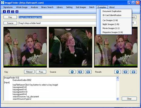
Figure 6.1 Example Menu.
In this chapter, we will introduce several examples. The number of image in each problem is around 1000.
6.1 Finding Duplicated Documents
Click menu item “Example/Document Duplication”, then click “Batch/Load”; this will load the example. This setting will also change the internal setting a bit. Now, we will walk through the Document duplication example.
Recent
developments in scanner technology have made it very easy to convert paper
documents into digital documents. A simple scanner can scan and save multiple
pages in a single click. The scanner
creates image names via auto-numbers you have specified.
This chapter attempts to solve a particular problem: to retrieve duplicated Document images. Assume you have a million pages of documents already converted into digital form, and you want to retrieve documents that meet some specified constraints. A typical Document retrieval system should have several components:
- Text;
- Image;
- 1-D barcode; and
- 2-D barcode.
Each component addresses a particular area of retrieval and their functions generally do not overlap. A complete solution should use all of the above options. This software deals with the image matching only.
6.1.1 Why Image Matching?
Image matching deals with several particular problems, which cannot be addressed by text search, 1D barcode search, or 2D barcode search:
(1) Tables: image matching
is responsible for retrieving documents with similar Tables.
Figure 6.2 Documents with Tables.
(2) Images: image matching is responsible for retrieving documents with similar images.
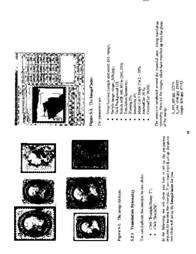
Figure 6.3 Documents with images.
(3) Special Symbols: image matching is responsible for retrieving documents with similar Special Symbols.
Figure 6.4 Documents with Special Symbols.
(4) Figures, Drawing, Designs:
image matching is responsible for retrieving documents with similar Figures,
Drawing, and Designs.
(5) Maps: image matching
is responsible for retrieving documents with similar Maps.
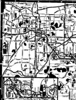
Figure 6.6 Documents with maps.
(6) Hand Written Notes: image matching
is responsible for retrieving documents with Hand Written Notes.

Figure 6.7 Documents with handwritten notes.
(7) …
6.1.2 Data
The data is located in the following folder:
Name Location # of Images * number of copies
Misc .\sp_document\misc\ 93 x 2 = 186
BioAPI .\sp_document \bioapi\ 119 x 3 = 357
Abm54 .\sp_document \abm54\ 160 x 3 = 480
Total 1,023 images
The “Misc” example has 93 matching pairs, or 186 images. It has various types of documents such as Tables, Images, Music, Figures, Drawings, Designs, Maps, …
The “BioAPI” example has 119 matching triplets, or 357 images. BioAPI is a document, which attempts to set up a standard for the biometric templates. This document has 119 pages.
The “Abm54” example has 160 triplets, or 480 images.
Positive Match
· The “Misc” example has 93 matching pairs, or 186 images; there are 186*2 positive matches.
· The “BioAPI” example has 119 triplets, or 357 images; there are 357*3 positive matches.
· The “Abm54” example has 160 triplets, or 480 images; there are 480*3 positive matches.
· In the file, “.\data\b1_matchlist_ex_doc.txt”, which is the summation of all positive matches, there are 186*2 + 357*3 + 480*3 = 2883 positive matches.
6.1.3 Signature
To select images and get the signature file:
- Click menu item “Example/Document Duplication”;
- Click “Batch/Load”.
At this point, the signatures for this problem are ready in a1.txt. Alternatively, you can start from beginning, to select images:
- Click the “Source” button to select directory, “.\sp_document\”.
To compute the N-signatures:
- Click “Signature/N Signature (a1.txt)” to compute the signatures in a1.txt.
This will take about some time.
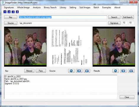
Figure 6.8 Click menu item “Example/Document Duplication”, then click “Batch/Load”; this will load the example.
6.1.4 Matching
N: N Matching compares each image, a1.txt, with every image in the a1.txt:
- Click menu item “Example/Document Duplication”;
- Click “Batch/Load” to load parameters;
- Click menu item “Whole Image/ N:N Matching (a1.txt vs. a1.txt)” to complete a N:N Match.
The results will go to a file, b1.txt, which will be opened right after the click. The file will look like this:
.\sp_document\abm54\abm54_a_0001.jpg
.\sp_document\abm54\abm54_a_0001.jpg
100
.\sp_document\abm54\abm54_a_0013.jpg
82
.\sp_document\abm54\abm54_a_0018.jpg
81
.\sp_document\abm54\abm54_a_0024.jpg
81
.\sp_document\abm54\abm54_a_0038.jpg
82
…
Total Number of Matches = 30317
6.1.5 Analysis
Possible Matches
Let the Total Images in the input file be N, the Possible Matches will be N*N. In our example,
T = N * N = 1023 x 1023 = 1,046,529.
Attrasoft Matches
The number of retrieved matches is listed in the last line of b1.txt. Go to the end of b1.txt, you will see something like this:
Total Number of Matches = 30317
Actual Match
This number
depends on your problem. It should be the first number in b1_matchlist.txt. In
our example, it is 2883.
Attrasoft Found Duplicates
To check the results, we must prepare the
b1_matchlist.txt file now. This file is already prepared for you; we will
simply open it and save it to b1_matchlist.txt (overwrite the existing file).
The steps are:
· Open “./data/b1_matchlist_ex_doc.txt. Save it to b1_matchlist.txt (overwrite the existing file). Now this file is prepared.
· Click “Analysis/Check (b1_matchlist.txt required)” to check the results.
The result is:
Total Matches = 2843
Now that you have all of the numbers, you can make an analysis.
Positive Identification Rate
Positive
Identification Rate = 2843/2883 = 98.6%.
Elimination Rate
Elimination Rate = (1 – (30317 – 2843)/1,046,529 = 97.4 %
Hit Ratio
The Hit
Ratio = 2843/30317 = 9.4 %.
Composite Index
The composite index is = 0.09.
We will improve the result with training.
6.2 Face Recognition
Click menu item “Example/ID Card Identification”; then click “Batch/Load”, and this example will be loaded.
This chapter attempts to solve a particular problem: to scan a document (passport, ID card, …) with a Face Photo ID and match this face image against an existing database. Assume you have millions of Photo ID’s already converted into images, and you want to make a 1:N Matching with the newly captured image.
6.2.1 Data
The data is located in the following folder:
.\sp_face\.
There are 516 pairs, or 1032 images. Each image will match itself and its partner; giving a total of 1032 * 2 = 2064 matches.
6.2.2 Signature
To compute the N-signatures:
- Click “Signature/N Signature (a1.txt)” to compute the signatures in a1.txt.
6.2.3 Matching
N: N Matching compares each image, a1.txt, with every image
in the a1.txt:
- Click menu item “Whole Image/N:N Matching (a1.txt vs. a1.txt)” to complete a N:N Match.
The results will go to a file, b1.txt, which will be opened right after the click. The file will look like this:
.\sp_face\00019ba010_960521.jpg
.\sp_face\00019ba010_960521.jpg
100
.\sp_face\00019bj010_960521.jpg
85
.\sp_face\00611fa010_940307.jpg
82
.\sp_face\00862fb010_940307.jpg
82
.\sp_face\00870fa010_940307.jpg
82
.\sp_face\01043bj010_960521.jpg
82
.\sp_face\01162ba010_960521.jpg
82
.\sp_face\01179ba010_960521.jpg
82
.\sp_face\00019bj010_960521.jpg
.\sp_face\00019ba010_960521.jpg
85
.\sp_face\00019bj010_960521.jpg
100
.\sp_face\00611fa010_940307.jpg
82
.\sp_face\00862fa010_940307.jpg
82
…
Total Number of Matches = 12640.
6.2.4 Analysis
Possible Matches
Let the Total Images in the input file be N, the Possible Matches will be N*N. In our example, N * N = 1032 x 1032 = 1,065,024.
Attrasoft Matches
The number of retrieved matches is listed in the last line of b1.txt. Go to the end of the file, b1.txt; you will see something like this:
Total Number of Matches = 12640.
Actual Match
This number depends on your problem. It should be the first number in b1_matchlist.txt. In our example, it is 2064.
Attrasoft Finds Matches
To check the results, we must prepare the
b1_matchlist.txt file now. This file is already prepared for you and we will
simply open it and save it to b1_matchlist.txt (overwrite the existing file).
The steps are:
· Open “./data/b1_matchlist_ex_face.txt. Save it to b1_matchlist.txt (overwrite the existing file). Now this file is prepared.
· Click “Analysis/Check(b1_matchlist.txt required)” to check the results.
The result is:
Total Matches = 1620
Now that you have all of the numbers, you can make an analysis.
Positive Identification Rate
Positive
Identification Rate = 1620/2064 = 78.5%.
Elimination Rate
Elimination Rate
= 1 – (12640 – 1620) /1,065,024 = 98.9%.
Hit Ratio
The Hit
Ratio = 1620/12640 = 12.8 %.
Composite Index
The composite index is = .1.
We can improve the result with training.
7. Binary Search
For a large amount of images, say above 1 million images, binary search is much faster. However, binary search requires additional steps, signature sorting and signature management. The “Binary Search” menu is given in Figure 7.1.
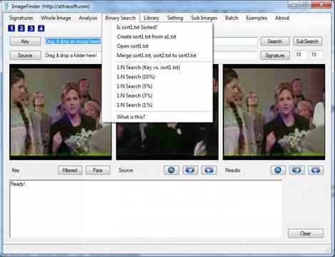
Figure 7.1 Binary Search Menu Items.
The search steps are:
1. Select a folder (Click the “1” Button in
the Toolbar, see Figure 4.2)
2. Get Library Signatures (Click the “2”
button in the Toolbar, see Figure 4.2)
3. Sort Signature (see Figure 7.1).
4. Select a Key image (Click the “3” Button
in the Toolbar, see Figure 4.2).
5. Search (There are several options in
Figure 7.1).
7.1 Signatures
For binary search, the signature file is sort1.txt. Unlike sequential search, which allows many signature files to be loaded via a library, the sorted signatures will use one single file, so you have to manage this file.
To get a signature file sort1.txt:
1. Select a folder (Click the “1” Button in
the Toolbar, see Figure 4.2).
2. Get Library Signatures (Click the “2”
button in the Toolbar, see Figure 4.2).
3. Click menu item Binary Search/Create
sort1.txt from a1.txt.
If you have several signature files, you have to merge them:
- Create sort1.txt;
- Copy sort1.txt to sort2.txt;
- Create sort1.txt with new data;
- Merge sort1.txt and sort2.txt to
sort3.txt.
The merger will be done by clicking “Binary Search/Merge sort1.txt, sort2.txt to sort3.txt”.
7.2 Search
To make a search:
- Select a Key image (Click the “3” Button
in the Toolbar, see Figure 4.2).
- Search.
There are several search options:
- Binary Search/1:N Search (key vs. sort1.txt)
- Binary Search/1:N Search (10%)
- Binary Search/1:N Search (5%)
- Binary Search/1:N Search (3%)
- Binary Search/1:N Search (1%)
Assume you have 1 million images, the first command above will search 1 million images; the second command will search 100 thousand images; the third command will search 50 thousand images; the fourth command will search 30 thousand images; and the last command will search 10 thousand images. By definition, the Binary Search will only ignore the parts that are not likely to yield a match.
Assume you use Sequential Search (Chapter 4) for 1 million images, you will search through 1 million images. Then you use the “Binary Search/1:N Search (1%)” for the same 1 million images, provided the image signatures are sorted, you will search through only 10 thousand images. The difference is a factor of 100.
Binary Search is more restrictive than 1:N whole image matching; so the two image search results do not always match. In general, Binary Search generates less results than 1:N while image matching.
8. Dynamic Library
In the last a few chapters, we introduced 1:N Match and N:N Match, where the N-Signature file is fixed. This chapter will introduce the Dynamic Library where the search library can be updated via insertion, deletion, and modification.
The first advantage of the Library is to load the library only once for all 1:N matching. The 4-step 1:N matching process introduced earlier loads the library for each matching. The cost of loading the library only once is two additional clicks:
- Create a library file;
- Load the library.
The second advantage is the library can be modified via insertion, deletion, and modification.
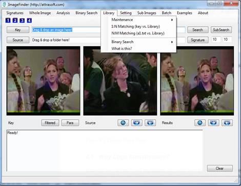
Figure 8.1 Library Menu Items
8.1 Image Signatures
We will use the wheel rim example. The data is located in the following folder:
.\ex_wheel\ Original logo data
.\ex_wheel_add\ Add to the library later
To compute the N-signatures:
- Click the “Source” button to select directory, “.\ex_wheel\”;
- Click “Signature/N Signature (a1.txt)” to compute the signatures in a1.txt.
8.2 Dynamic Library
To use the Dynamic Library, you have to create a library from file lib1.txt, so the first two things we will do are:
- Create lib1.txt;
- Load the library, lib1.txt.
To create a library file, lib1.txt, click “Library/Maintenance/Create lib1.txt from a1.txt”.
To load the library file, click “Library/Maintenance/Load lib1.txt”.
8.3 Library 1:N Matching
To make 1:N Matching via
the library,
·
Click the “Key”
button, in the “ex_wheel” directory, select the first image “2067(1).jpg”;
·
Click menu item
“Library/1:N Matching (Key vs. lib1.txt)” to complete a 1:N Match.
8.4 Library N:M Matching
In
an N:M Matching, the N-images are in a1.txt and M-images are in lib1.txt. To
make a N:M Matching,
·
Click menu item “Library/N:M Matching(a1.txt vs. lib1.txt)” to complete
a N:M Match.
8.5 Library Updating
Now,
we will add images in folder, “.\ex_wheel_add\”. To make 1:N Matching via the
library,
·
Click the “Key” button, in the “.\ex_wheel_add\” directory; select the
image “1er_1.jpg”;
·
Click menu item “Library/Matching/1:N Matching (Key vs. lib1.txt)” to
complete a 1:N Match.
You will get:
No
Match!
To add this image to the library, click:
“Library/Maintenance/Add (Key)”.
Now, make a 1:N Match again:
·
Click menu item “Library/Matching/1:N (Key vs. lib1.txt)” to complete a
1:N Match.
You will get Figure 8.2:
ID Name Path Score X Y W H
1er_1 1er_1.jpg .\ex_wheel_add\ 100 0 0 0 0 …
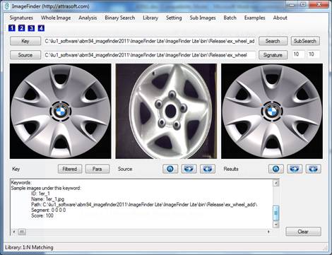
Figure 8.2 Add an image signature to the in-memory library.
As you can see, 1er_1.jpg has been added to the library.
Now we will delete it from the library by clicking:
“Library/Maintenance/Delete (Key)”.
Now make a 1:N Match again:
· Click menu item “Library/ 1:N Matching (Key vs. lib1.txt)” to complete a 1:N Match.
Now 1er_1.jpg will no longer be in the output.
8.6 Load Multiple Libraries and Additional Libraries
After loading the first library, .\data\lib1.txt, you can load one additional library:
- Click “Library/Maintenance/Load Additional(lib2.txt)”.
You can load multiple libraries. The library files must be stored in the folder, .\data\libraries\. To load:
- Click “Library/Maintenance/Load Library (.\data\libraries\*.txt)”.
After initial loading, you can load additional libraries:
- Click “Library/Maintenance/Load Additional Library (.\data\librariess\*.txt)”.
8.7 Binary Search
The Library Menu also supports binary search, see Figure 8.2. These menu items work similar to the Binary Search menu items.
The library will load from a single sorted library sort1.txt and make 1:N search.
Binary Search is more restrictive than 1:N whole image matching; so the two image search results do not always match. In general, Binary Search generates less results than 1:N while image matching.
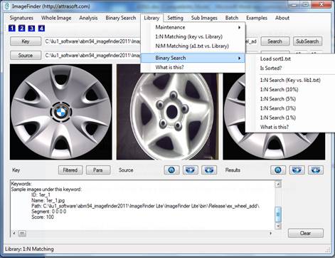
Figure 8.3 Library/Binary Search menu items.
9. Sub Image Search
The sub image matching requires a different set of parameters. There are two different settings:
Setting/Search Sub Images
Setting/Search Whole Images
To match sub images, click menu item, “Setting/Search Sub Images”. To switch back to the original setting for whole image, click: “Setting/Search Whole Images”.
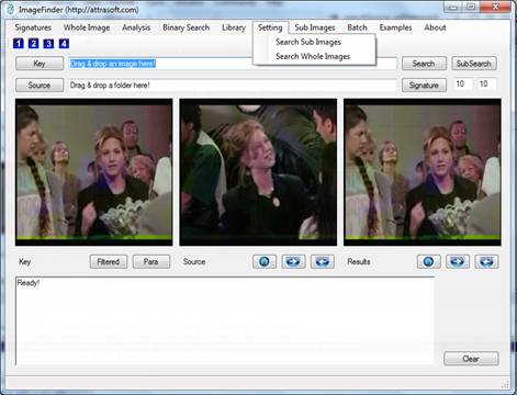
Figure 9.1 Setting Change.
9.1 Sub Images and Variations
Starting from this chapter, we will search inside an image. We will deal with the problems of:
- Sub image
- Variations.
The number of sub images is very large, measured by exponential functions of the number of pixels. The number of variations is also very large:
- Translated segments;
- Rotated segments;
- Scaled segments;
- Rotated and Scaled segments;
- Brighter or Darker segments;
· ...
- All of the above simultaneously.
We will not use image signatures because of the large amount of variations. This will significantly slow down the search speed.
Because the variations for searching inside an image are huge, we might impose some limits on where to search. There are several approaches:
- Automatic Segmentation;
- Enumerative.
Automatic segmentation deploys certain algorithms to look at a small number of segment locations inside the image. There are two menu items to address this approach (Chapter 3):
The “Signature/Segment Signatures” menu item (Figure 3.1) computes signatures for a selected number of image segments. The net result is that an image will have multiple image signatures, one for each segment.
The “Signature/Segment Image” menu item (Figure 3.1) will compute segment images from the key image and will deposit them into “.\tmp\” folder. To use this menu item, you must first select a key image. This allows a user to see what the segments are.
The advantages of automatic segmentation are that it will dramatically reduce the number of search locations. The disadvantages of segmentation algorithms are that it will not be able to address some human cropped images which cut right through the middle of a segment.
The enumerative approaches are not restricted by the automatic segmentation algorithm; however, the variations for enumerative sub image searching are huge; some sort of limits on where to search will have to be imposed.
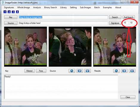
Figure 9.2 Two parameters.
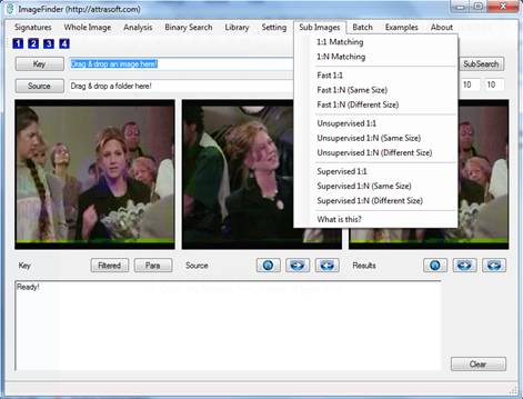
Figure 9.3 Sub Image Menu.
9.2 Search Process
In this chapter, we will use enumerative search by imposing these two conditions:
- Translation invariance only;
- No scale, rotation, …, invariance.
In each search, there are two parameters N x M (Figure 9.2), which
specify an array of sub-images to search. The software will search via an “N by
M” grid for each unknown image for the specified key image. The key will not be
rotated or scaled.
Initially, you will need three steps for an image search:
1. Select a Key;
2. Select a folder;
3. Search.
To see the results:
1. Click the Results Home button (Figure 9.3);
2. Click the Results “=>” button (Figure
9.3).
Starting from the second search, you do not have to select the folder
again because it is already selected; each search has only two steps:
1. Select a Key;
3. Search;
1. Select a Key;
3. Search;
…
Note:
Step 1, selecting a Key can be completed by
dragging & dropping an image to the first text box;
Step 2, select a folder, which can be
completed by dragging & dropping a folder to the second text box.
9.3 Learn by Example
There are several examples in the software:
.\ ex_object1\
.\ ex_object2\
.\ ex_object3\
.\ ex_object4\
.\ ex_object5\

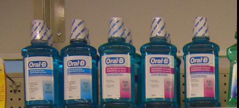
Figure 9.4 1:1
Matching.
The first example (see Figure 9.4) is to match the key,
.\ ex_object1\key.jpg,
against the image,
.\ ex_object1\CIMG4643_mid_shelf1.JPG.
The example will take three clicks:
1.
Click
the “Key” button in the Toolbar, and select .\ ex_object1\
key.jpg. You can also drag & drop .\ ex_object1\key.jpg to the first text
box.
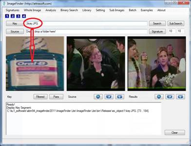
Figure 9.5 Step 1, selecting a key. After selecting a key image, the image will be displayed in the Key Panel.
2.
Click the “Source” button in the Toolbar
and select the folder, .\
ex_object1\.
You
can also drag & drop the folder, .\ ex_object1\,
to the second text box; the use “=>’ button to select image, .\
ex_object1\CIMG4643_mid_shelf1.JP, see
Figure 9.6.
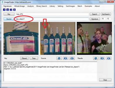
Figure 9.6 Step
2, selecting a folder. After selecting a folder, the first image will be
displayed in the Source Panel (middle picture box). The list of image files
will be displayed in the text window. The Home button goes to the first image;
the “=>” button goes to the next image; and the “<=” button goes to the previous image. All sub-folders
will be included.
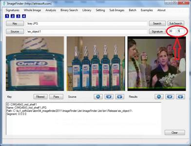
Figure 9.7 Search
the N x M grid of sub-images. For example, setting them to 30 x 5 will result
in searching 150 sub-images.
3.
Before we make a search, you will
specify how to search via an “N by M” grid, i.e. how many sub-images we will
look at for the specified key image. The default value is a 10 by 10 grid.
To
make a 1:1 search,
·
Enter 30 and 5 in Figure 9.7.
·
Click the “Sub Image/1:1 Matching” menu
item in Figure 9.3.
You
will get:
ID Name Path Score X Y W H
CIMG4643_mid_shelf1.JPG_146 CIMG4643_mid_shelf1.JPG .\ex_object1\ 84 366 34 73 184
CIMG4643_mid_shelf1.JPG_134 CIMG4643_mid_shelf1.JPG .\ex_object1\ 84 197 34 73 184
CIMG4643_mid_shelf1.JPG_123 CIMG4643_mid_shelf1.JPG .\ex_object1\ 83 42 34 73 184
CIMG4643_mid_shelf1.JPG_110 CIMG4643_mid_shelf1.JPG .\ex_object1\ 83 282 25 73 184
CIMG4643_mid_shelf1.JPG_117 CIMG4643_mid_shelf1.JPG .\ex_object1\ 81 380 25 73 184
CIMG4643_mid_shelf1.JPG_100 CIMG4643_mid_shelf1.JPG .\ex_object1\ 80 141 25 73 184
Note,
if you do not get this, click menu item, “Setting/Search Sub
Images” and then try again.
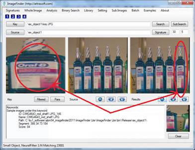
Figure 9.8
Search the selected folder. Images that matched the “key”
will be displayed in the Results Panel. Use the Home, =>, and <=buttons
to see matched images. The Home button goes to the first image; the “=>”
button goes to the next image; and the “<=”
button goes to the previous
image.
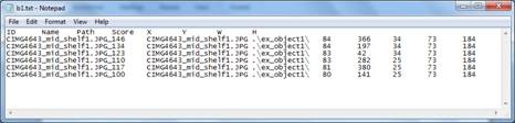
Figure 9.9
The matched score and coordinates,
(x, y, w, h), are given in a text file: “.\data\c.txt”.
To see the first matched image, click the Home button in the Results Panel (see Figure 9.8). To see the next matched image, click the “=>” button in the Results Panel. The key and the matched images are displayed side-by-side.
9.4 User’s Guide
1. Select a Key
A key is a cropped image segment you are looking for from a folder. You can create a key from an image, see Figure 9.4.
This step selects a key by:
· Clicking the “Key” button, or
· Dragging and dropping an image into the first textbox.
The selected key will be displayed in the first picture box.
2. Select a Source
This step selects an image folder that has images you want to search through. This step is implemented by:
· Clicking the “Source” button, or
· Dragging and dropping a folder into the second textbox.
The images in the selected folder will be displayed in the second picture box. Use the Home button to select the First image in the folder; use the “=>” button to select the next image; and use the “<=” button to select the previous image.
3A. 1:1 Search
This step has two parameters: N, M, which specifies an array of sub-images to search. The software will search from an N by M grid for the key image. To search:
·
Click the “Sub Image/1:1 Matching” menu item.
To see the results:
1. Click the Results Home button;
2. Click the Results “=>” button.
3B. 1:N Search
This step has two parameters: N, M, which specifies an array of sub-images to search. The software will search all images from a folder. For each image, the software will search from an N by M grid for the key images. This step is implemented by clicking:
·
Click the “Sub Image/1:N Matching”
menu item.
To see the results:
1. Click the Results Home button;
2. Click the Results “=>” button.
Comments:
·
The key image will not be scaled.
·
The key image will not be rotated.
9.5 Example 2
There are more examples in the software:
.\ ex_object1\
.\ ex_object2\
.\ ex_object3\
.\ ex_object4\
.\ ex_object5\
The second example makes a 1:N
search. This example uses data in .\ ex_object2\.
·
Click
the “Example/Car Image (1:N)” menu item to complete steps 1 and 2;
·
Click
the “Sub Image/1:N Matching” menu item.
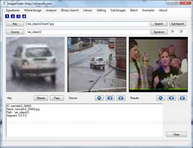
Figure 9.10 Click the “Example/Car Image” menu item to
start Example 2.
The results are given in Figure 9.11 and Figure 9.12.
Figure 9.11shows a blue box over the image segment that has matched
with the key.
Figure 9.12 shows the coordinates (x, y w, h) of the matched segments,
where (x, y w, h) = (Left, Top, Width, Height).
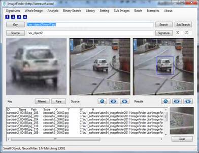
Figure 9.11 Example
2 results.
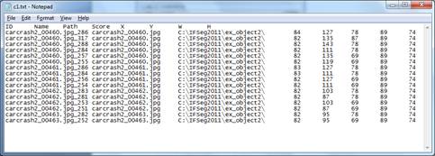
Figure 9.12 Example
2 results.
9.6 Example 3
To start Example 3:
·
Click the “Example/Night Image” menu
item;
·
Click the “Sub Image/1:N Matching”
menu item.
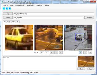
Figure 9.13 Click
“Example/Night Images” menu item to load Example 3.
The results are given in Figure 9.14 and Figure 9.15.
Figure 9.14 shows a blue box over the image segment that has matched
with the key.
Figure 9.15 shows the coordinates (x, y w, h) of the matched segments,
where (x, y w, h) = (Left, Top, Width, Height).
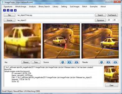
Figure 9.14 Example 3 results.
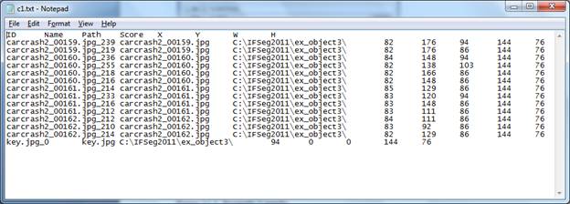
Figure 9.15 Example 3 results.
9.7 Example 4
To start Example 4:
·
Click the “Example/Movie Image” menu
item;
·
Click the “Sub Image/1:1 Matching ”
menu item.
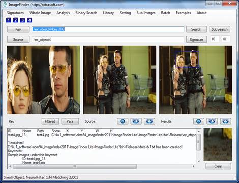
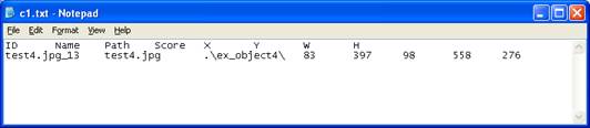
Figure 9.16 Click
“Example/Movie Images (1:1)” menu item to load Example 4. The result is shown
in the blue box in the third image.
9.8 Large Image: Example 5
To deal with larger images, say above 1000x1000, the ImageFinder uses a different set of parameters.
In order for you to process large images, you should start with clicking the “Example/Magazine Image (1:1)” menu item, which loads the parameters for larger images.
To start Example 5:
·
Click the “Example/Magazine Image
(1:n)” menu item;
·
Click the “Sub Image/1:N Matching ”
menu item.
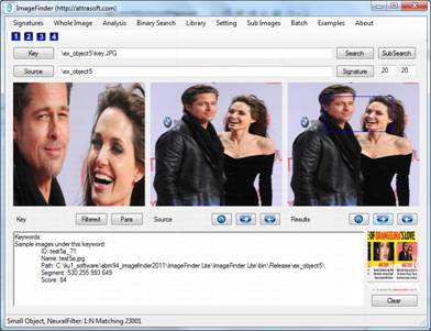
Figure
9.17 Click
the “Example/Magazine Image (1:N) ” menu item to start Example 5. There are two
magazine images in this example.
10. Sub Image Part II
The sub image matching requires a different set of parameters. There are two different settings:
Setting/Search Sub Images
Setting/Search Whole Images
To match sub images, click menu item, “Setting/Search Sub Images”. To switch back to the original setting for whole images, click: “Setting/Search Whole Images”.
The objective for the last chapter menu is to find a cropped segment at
all cost, provided there is no scaling factors. This can take a long time if
the N x M search grid is set to be very large. The first objective of this
chapter is to find a cropped segment much faster. The second objective is to
add scale invariance and rotation invariance.
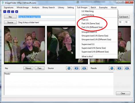
Figure 10.1 “Fast” menu items.
10.1 Fast Menu
The objective of the “Fast” menu items is to find a cropped segment
from an image within 1 second.
The “Fast” menu items provide a much faster search than the menu items
of the last chapter, but these menu items are less accurate than those in the
last chapter. It is a trade-off between accuracy and computation time. Figure
10.1 shows the menu items under this menu.
Example. We will match (see Figure 9.4 from last
chapter) the key,
.\ ex_object1\key.jpg,
against the image,
.\ ex_object1\CIMG4643_mid_shelf1.JPG.
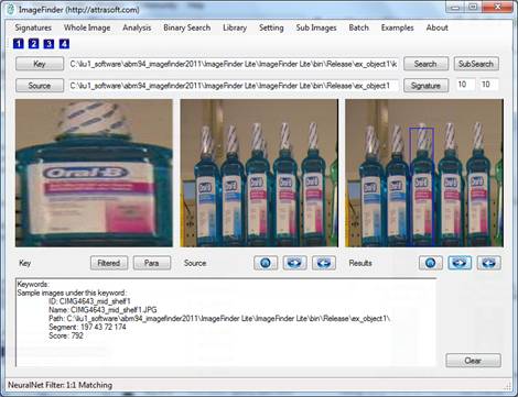
Figure 10.2 Fast match results.
Before starting this example, click menu item, “Setting/Search Sub Images”.
The example will take three clicks:
1.
Click the “Key” button, and select .\ ex_object1\key.jpg.
You can also drag & drop .\ex_object1\key.jpg to the first text box.
2.
Click the “Source” button and select
the folder, .\ ex_object1\. You can also drag & drop the folder, .\ ex_object1\,
to the second text box.
3.
Fast Search.
Click Fast/1:1 Matching and see the result in Figure 10.2.
The menu items are given below:
Sub Image/Fast 1:1
Use “Sub
Image/Fast 1:1” to make a 1:1 Matching.
Sub Image/Fast 1:N (Same size)
Use “Sub Image/Fast 1:N (Same size)” to make a 1:N Matching; it will
search through all images in a folder for the specified cropped image. This
command is faster than “Sub Image/1:N (Different size)”, but it requires all images in the search folder to
have the same pixel size.
Sub Image/Fast 1:N (Different
size)
Use “Sub Image/Fast 1:N (Different size)” to make a 1:N Matching; it
will search through all images in a folder for the specified cropped image.
This command is slower than “Sub Image/1:N (Same size)”, but it does not requires all images in the search folder
to have the same pixel size.
10.2 Unsupervised Menu
The objective of the “Unsupervised” menu is to find a cropped segment
from an image in 10 seconds.
The “Unsupervised” menu items works similar to the “Fast” menu items;
it provides a much faster search those in the than last chapter, but this menu
is less accurate. It is a trade-off between accuracy and computation time.
“Unsupervised” Menu is more accurate than the “Fast” Menu, but slower than the
last chapter. Figure 10.1 shows the menu
items under this menu.
Example. We will match the key,
.\ ex_object1\key.jpg,
against the image,
.\ ex_object1\CIMG4643_mid_shelf1.JPG.
The example will take three clicks:
1.
Click
the “Key” button, and select .\ ex_object1\key.jpg.
You can also drag & drop .\
ex_object1\key.jpg to the first text box.
2.
Click
the “Source” button and select the folder, .\ ex_object1\.
You can also drag & drop the
folder, .\ ex_object1\, to the second text box.
3. Search.
Click Fast/1:1 Matching and see
the result.
The menu items are given below:
Sub Image / Unsupervised 1:1 Matching
Use “Sub Image / Unsupervised 1:1 Matching”
to make a 1:1 Matching.
Sub Image /Unsupervised /:N Matching (Same size)
Use “Sub Image /Unsupervised /:N Matching
(Same size)” to make a 1:N Matching; it will search through all images in a
folder for the specified cropped image. This command is faster than
“Unsupervised /1:N Matching (Different size)”, but it requires all images in
the search folder to have the same pixel size.
Sub Image / Unsupervised 1:N Matching (Different size)
Use “Sub Image / Unsupervised 1:N Matching
(Different size)” to make a 1:N Matching; it will search through all images in
a folder for the specified cropped image. This command is slower than
“Unsupervised/1:N Matching (Same size)”, but it does not requires all images in
the search folder to have the same pixel size.
10.3 Supervised Menu
The objective of the “Supervised” menu is to find a cropped segment
from an image in 10 seconds.
The “Supervised” menu items works similar to the “Fast” menu items; it
provides a much faster search than those in the last chapter, but this menu is
less accurate. It is a trade-off between accuracy and computation time.
“Supervised” Menu is more accurate than the “Unsupervised” Menu; but slower
than the “Unsupervised” Menu. Figure 10.1 shows the menu items under this menu.
Example. We will match the key,
.\ ex_object1\key.jpg,
against the image,
.\ ex_object1\CIMG4643_mid_shelf1.JPG.
The example will take three clicks:
1.
Click the “Key” button, and select .\ ex_object1\key.jpg.
You
can also drag & drop .\ ex_object1\key.jpg to the first text box.
2.
Click the “Source” button and select
the folder, .\ ex_object1\.
You
can also drag & drop the folder, .\ ex_object1\, to the second text box.
3.
Search.
Click Fast/1:1 Matching and see the result.
The menu items are given below:
Sub Image /Supervised 1:1 Matching
Use “Sub Image /Supervised 1:1 Matching” to
make a 1:1 Matching.
Sub Image / Supervised 1:N Matching (Same size)
Use “Sub Image / Supervised 1:N Matching
(Same size)” to make a 1:N Matching; it will search through all images in a
folder for the specified cropped image. This command is faster than “Supervised
/1:N Matching (Different size)”, but it requires all images in the search
folder to have the same pixel size.
Sub Image / Supervised 1:N Matching (Different size)
Use “Sub Image / Supervised 1:N Matching
(Different size)” to make a 1:N Matching; it will search through all images in
a folder for the specified cropped image. This command is slower than
“Supervised/1:N Matching (Same size)”, but it does not requires all images in
the search folder to have the same pixel size.
11. Image Preprocessing
Up to this point, you have been using the default parameters. From this point on, you can change the behavior of the ImageFinder. There are two ways you can change the ImageFinder:
- Tweaking;
- Retraining.
Tweaking should be your first option; if that still does not work well, you can retrain the ImageFinder from the beginning.
If your new setting does not work well, please reinstall the ImageFinder to restore the old setting.
(1) Tweaking
For the ImageFinder, the Image Matching is divided into:
Image Preprocessing
Image Processing
Normalization
Image Signatures
Signature Matching
Subimage Matching
One or more filters further implement each
step. For the beginners, Image Preprocessing, Image Processing, and
Normalization can be set by default. There are over 100 parameters that can be
adjusted.
(2) Retraining
The ImageFinder is trained, not programmed. The ImageFinder depends on its training. Currently, the ImageFinder is trained with 10,000 pairs of random images. You can change the how the ImageFinder behaves by training the ImageFinder from beginning.
Attrasoft ImageFinder learns an image in a way similar to human eyes:
- Ignore the background;
- Focus on an object in the image.
The image preprocessing in this chapter and the image processing in the next chapter prepare the image for the ImageFinder. The image processing process is not unique; there are many options available. Some are better than others.
The principle of choosing the image preprocessing and processing filters is to make the sample objects stand out, otherwise change the options.
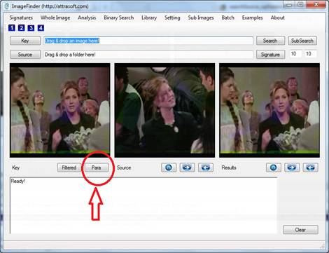
Figure 11.1 “Para” button.
Image preprocessing has the following functions:
- Cut off the border areas;
- Impose a mask;
- Speed up the computation;
- Skip the empty border areas;
Do not make too many things stand out, i.e. as long as the area of interest stands out, the rest should show as little as possible.
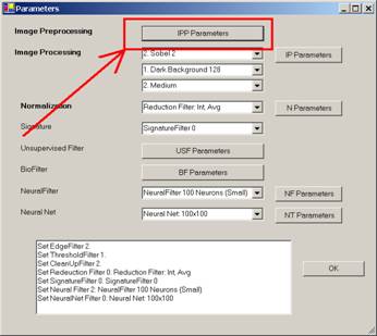
Figure 11.2 Image
preprocessing filter in the Parameter Window.
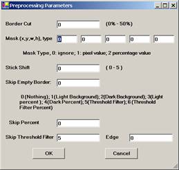
Figure 11.3 Image
Preprocessing.
To see the current
image preprocessing filter, first select a key image, then click the “Filtered”
button under the key picture box. Clicking the button again will restore the
original image.
11.1 Set Image Preprocessing Filter
To
set the Image-Preprocessing Filter, click the “Para” button (see Figure 11.1)
to get Figure 11.2. Click the “IPP (Image PreProcessing) Parameters” button in
Figure 11.2, you will see Figure 11.3. You will set the Image-Preprocessing
Filter on Figure 11.3.
To see the effect of the image preprocessing and image processing filters, click the “Filtered” button; you will see Figure 11.4. Clicking the button again will restore the original image.
11.2 Cut Off the Border Areas
Let us assume we want to cut off 10% of the border, enter 10 to the first textbox in Figure 11.3. Figure 11.4 shows the effect of cutting out the borders.
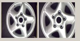
Figure 11.4a Five
Percent Border Cut on each side.
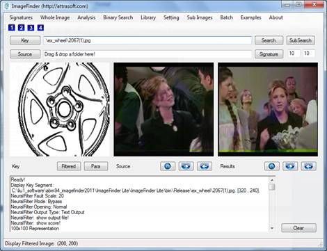
Figure 11.4b Five
Percent Border Cut on each side. To see the current image preprocessing
filter, click the “Filtered” button. Clicking the button again will restore the
original image.
11.3 Impose a Mask
Let us assume we want to cut off 20% of the border on top, 20% on the left, 10% on the right, and 10% on the bottom, then enter (x, y, w, h, type) = (20, 20, 70, 70, 2) to the second row textboxes in Figure 11.3 and we will have 11.5.
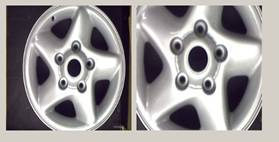
Figure 11.5 Mask
(20, 20, 70, 70, 2).
Now, if we use pixels rather than percentage, enter (20, 20, 70, 70, 1) to the second row textboxes in Figure 11.3 and we will have 11.6.
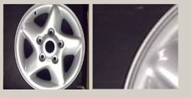
Figure 11.6 Mask (20, 20, 70, 70, 1).
11.4 Speed Up the Computation
To speed up the computation, set the parameter “Stick Shift” in Figure 11.2 between 0 and 5, with 0 being the slowest and 5 being the fastest.
11.5 Skip the Empty Border by Content Percent
The last function for the Preprocessing filter is to skip border by content percent, not pixel percent.
The “Skip Empty Border” field in Figure 11.3 specifies the type:
0 No skip;
1 Skip the white empty border space;
2 Skip the black empty border space;
3 Skip x percent of the contents on the white background space;
4 Skip x percent of the contents on the black background space;
5 Skip empty border space on the user defined Threshold Filter;
6 Skip x percent of the contents on the user defined Threshold/Edge Filters.
We will discuss Threshold/Edge Filters in the next chapter, Image Processing.
Example 1. Set “Skip Empty Border” = 2, meaning skipping black empty space on the edge. The result is shown in Figure 11.7; you will see that the second image is the first image without a black border.
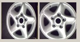
Figure 11.7 Skipping the black empty space.
Example 2. Set “Skip Empty Border” = 4, meaning skipping black empty space on the edge. Set “Skip percent” = 10 (meaning skipping 10% of the contents). The result is shown in Figure 11.8; you will see that the second image is the first image with 10% of the contents cut on each side.
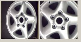
Figure 11.8 Skipping 10% of the contents on black background.
12. Image Processing
Attrasoft ImageFinder learns an image in a way similar to human eyes:
- Ignore the background;
- Focus on an object in the image.
The Image Preprocessing in the last chapter and the Image Processing in this chapter prepare the image for the ImageFinder.
The Image Processing process is not unique; there are many options available. Some are better than others. For many problems like fingerprints, palm prints, …, special image processing filters will be required.
12.1 Good & Bad
The principle of choosing the image preprocessing and processing filters are to make the sample objects stand out, otherwise change the options.
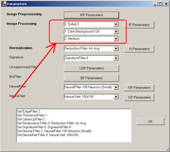
Figure 12.1 shows the default setting.
First of all, let us use the default setting:
Edge Filter = 2
Threshold Filter = 1
Clean-Up Filter = 2.
A second setting could be:
Edge Filter = 0
Threshold Filter = 1
Clean-Up Filter = 16
12.2 Set Image Processing Filters
The image processing will be applied to all images before recognition. As far as the operation is concerned, this means setting three filters:
Edge Filters;
Threshold Filters; and
Clean-Up Filters.
In Figure 18.1,
- to select an Edge Filter, click the Edge Filter Drop Down List, which is the first List in the red box;
- to select a Threshold Filter, click the Threshold Filter Drop Down List, which is the second List;
- to select a Clean-Up Filter, click the Clean-Up Filter Drop Down List, which is the third List.
The Edge Filters attempt to exaggerate the
main features a user is looking for.
The Threshold Filters attempt to suppress the
background.
The Clean-Up Filters will smooth the
resulting image to reduce recognition error.
The default setting is:
Edge Filter = 2
Threshold Filter = 1
Clean-Up Filter = 2
12.3 First Two Settings
The default
setting should be your first choice:
Edge Filter = 2 or “Sobel 2”.
Threshold Filter =1 or “Dark Background 128”.
Clean-Up Filter = 2
Your second
choice should be:
Edge Filter = 0
Threshold Filter =5
Clean-Up Filter = 2
To see the current
image preprocessing filter, first select a key image, then click the “Filtered”
button under the key picture box. Clicking the button again will restore the
original image.
13. Signature Filter
You can change the image signatures. The image signature is generated by image signature filters. Once you change the filters, you change the image signature. Figure 13.1 shows how to change the signature filter.
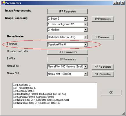
Figure 13.1 Parameter
Window.
The default setting uses the Signature Filter 16. There are 20 Signature filters in the current version of the ImageFinder. In general, when you have less data, use less accurate Signature filters; when you have more data, use more accurate Signature filters.
The reasons you might change the filters are:
- Reduce the image signature size;
- Increase Accuracy;
- Train the Whole Image matching filter from the beginning.
Figure 13.1 shows how to select a different signature filter; simply click the drop down list and select a new filter.
When you change the image signatures, the software has to be trained again. Please refer the training chapter to see how you can train the software for a new filter.
14. Batch Job
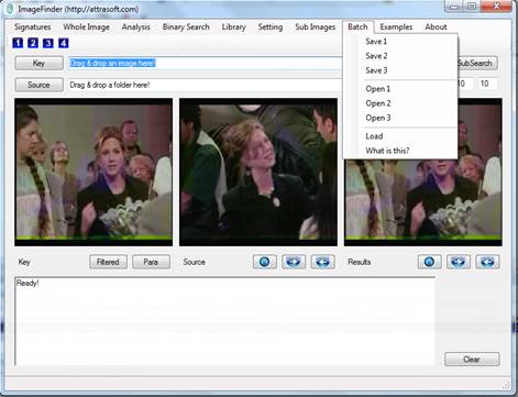
Figure 14.1 Batch Menu.
When matching images, you will need to select many filters. For each selected filter, you will need to select many parameters. Up to this point, you have been using the default values.
However, if you changed the parameters, you can save the parameters by clicking the "Batch/Save 1" menu item.
The Batch Process is:
(1) Create an application using the ImageFinder;
(2) Save the setting to a batch code with the following commands:
Batch/Save 1, or
Batch/Save 2, or
Batch/Save 3;
(3) Later, you can open the batch file with the following commands:
Batch/Open 1, or
Batch/Open 2, or
Batch/Open 3;
(4) To load the parameters without running, click:
Batch/Load.
The Batch/Save command saves the internal parameters.
15. Training
The whole image matching filter is called the Neural Filter. The Neural Filter will need to be trained before matching. Up to this point, the training has been using the default data.
You can train the Neural Filter yourself. The entire process will have four steps:
·
Signatures
·
Training
- Matching
- Analysis
Training teaches the ImageFinder what to look for. The Neural Filter training requires two files, t1.txt and match.txt:
- T1.txt is the signature file, which contains many signatures. Each image is converted into a signature.
- Match.txt is a list of matching pairs. This file will teach the ImageFinder who will match with whom.
Once you get the two files prepared, click “Whole
Image\Training\Training” to train the Neural Filter.
The more training pairs you have, the more accurate
the results will be. At minimum, you will need the number of matching pairs
specified as follows:
Signature Filter Training Pairs
0 10
1 30
2 30
3 70
4 70
5 150
6 150
7 310
8 310
9 630
10 630
> 11 1000
15.1 Document Matching Example
The ImageFinder training requires two files, t1.txt and match.txt:
· T1.txt is the signature file, which contains many signatures. Each image is converted into a signature.
·
Match.txt is a list of matching pairs. This file
will teach the ImageFinder who will match with whom.
To get the
N-signature file, a1.txt:
- Click the
“Source” button, select folder, “.\sp_document\”.
- Click the
Source “>” button a few times to see the images;
- Click menu
item “Signature/N Signature (a1.txt)” to get the signatures in a1.txt
file.
Match.txt
·
Open the file, “.\data\match_ex_doc.txt”. This file lists matching
pairs. Save it to match.txt (overwrite the existing file). Now the training
file is prepared.
T1.txt:
· Click menu item “Whole Image/Training/Copy a1.txt to t1.txt” to get the training file, t1.txt.
Note: Here t1.txt is for training and a1.txt is for 1:N Matching and N:N Matching.
Training
·
Click “Whole Image\Training\Training Without Saving” to train the ImageFinder.
Parameter
Set:
Neural
Filter è Threshold = 0.
N: N Matching compares each image, a1.txt, with every image in the a1.txt:
- Click menu item “Whole/N:N Matching (a1.txt vs. a1.txt)” to complete a N:N Match.
The result is:
Total Number of Matches = 3231.
Analysis
To check the results, we
must prepare the b1_matchlist.txt file now. This file is already prepared for
you and we will simply open it and save it to b1_matchlist.txt (overwrite the
existing file). The steps are:
· Open “./data/b1_matchlist_ex_doc.txt. Save it to b1_matchlist.txt (overwrite the existing file). Now this file is prepared.
· Click “Analysis/Check(b1_matchlist.txt required)” to check the results.
The result is:
Total Matches = 2883.
Analysis
Possible
Matches
Let the Total Images in the input file be N, the Possible Matches will be N*N. In our example,
T = N * N = 1023 x 1023 = 1,046,529.
Attrasoft
Matches
The number of retrieved matches is listed in the last line of b1.txt. Go to the end of b1.txt, you will see something like this:
Total Number of Matches = 3231
Actual Match
This number depends on your problem. It
should be the first number in b1_matchlist.txt. In our example, it is 2883.
Attrasoft Found
Duplicates
To check the results, we
must prepare the b1_matchlist.txt file now. This file is already prepared for
you and we will simply open it and save it to b1_matchlist.txt (overwrite the
existing file). The steps are:
· Open “./data/b1_matchlist_ex_doc.txt. Save it to b1_matchlist.txt (overwrite the existing file). Now this file is prepared.
· Click “Analysis/Check(b1_matchlist.txt required)” to check the results.
The result is:
Total Matches = 2883
Now that you have all of the numbers, you can make an analysis.
Positive Identification
Rate
Positive Identification Rate = 2883/2883 = 100%.
Elimination Rate
Elimination Rate = (1 – (3231 – 2883)/1,046,529 = 99.97 %
Hit Ratio
The Hit Ratio = 2883/3231 = 89.2 %.
Composite
Index
The composite index is = 0.89.
This number is increased by an order of magnitude, from 0.09 to 0.89.
16. Parameters
This chapter will describe the parameters in the ImageFinder.
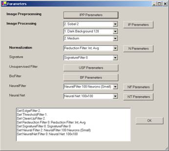
16.1 Overview
Attrasoft ImageFinder can:
· Match whole images;
· Match a portion of an image.
When matching a portion of an image, similar images are defined as images containing the sample segments, or:
- Translated segments;
- Rotated segments;
- Scaled segments;
- Rotated & Scaled segments;
- Brighter or Darker segments.
To match an image, the ImageFinder pushes the image through many filters. For example, a set of filters could be:
Preprocessing Filters
Edge Filters
Threshold Filters
Clean-Up Filters
Reduction Filters
Unsupervised Filters
NeuralFilters
NeuralNet Filters
Many parameters and options of the ImageFinder are hidden. The users have only limited control of the parameters. Still, the ImageFinder has many parameters, which can be adjusted by users. Click the “Para” Button; you will see Figure 16.1, where you can set the available parameters.
16.2 Image Preprocessing
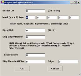
Use the “Stick Shift” parameter to speed up
the computation. Set “Stick Shift” in
Figure 16.2 between 0 and 5, with 0 being the slowest and 5 being the fastest.
0 No skip;
1 Skip the white empty border space;
2 Skip the black empty border space;
3 Skip x percent of the contents on the white background space;
4 Skip x percent of the contents on the black background space;
5 Skip empty border space on user defined Threshold Filter;
6 Skip x percent of the contents on user defined Threshold/Edge Filters.
16.3 Image Processing
16.3.1 Edge Filters
Edge
Filters extract and enhance edges & contours in an image by expressing
intensity differences (gradients) between neighboring pixels as an intensity
value. The basic variables are the differences between the top and bottom rows,
the differences between the left and right columns, and the differences between
the center point and its neighbors.
Edge Filters have the following selections:
Code Meaning
0 No Edge Filter
1 Sobel 1 (Prewitt)
2 Sobel 2 (Sobel)
3 Sobel 3
…
16.3.2 Threshold Filters
After Edge Filters, the Threshold Filter will be applied to images. Choose these two filters where the sample objects stand out, otherwise change the filters.
Once you make a selection, the objects in the images are black and the background is white (like a book: white paper, black print). You should make the black area as small as possible, as long as it covers the key-segment(s).
16.3.3 Clean-Up Filters
Clean-Up Filters will clear noise in the images, but it will take more computation time.
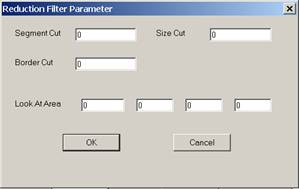
Figure 16.4 Selecting Reduction
Filter.
16.4 Normalization Filter
The Normalization Filter, also called Reduction Filter, connects the image to the underlying neural nets, 100x100 in size.
There are several ways to reduce images:
- Integer,
- Real, or
- All images are reduced by the same amount.
Integer Reduction
Images are reduced by an integer factor to maximally fit 100x100 without distortion. For example, a 350x230 image will be reduced to 87x57.
Real Reduction
Images are reduced by a real number to maximally fit 100x100 without distortion. For example, a 350x230 image will be reduced to 100x65.
Within each type of reduction, there are 3 more settings. Assume a 3x3 pixel array is reduced to 1 pixel,
- Avg: Assign the average of the 3x3 pixel array to the new pixel;
- Max: Assign the maximum of the 3x3 pixel array to the new pixel; or
- Min: Assign the minimum of the 3x3 pixel array to the new pixel.
To select the Reduction Filter, use the fourth drop down list. The Reduction Filter has seven parameters.
Segment Cut
This parameter deals with the edges of the segments in the images. The Segment Cut parameter ranges from 0 to 12. The larger this parameter is, the smaller the segment the ImageFinder will use. The possible settings in the user interface are: 0, 1, 2, .., and 12.
16.5 Neural Filter
Neural Filter is the filter for whole image matching.
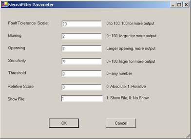
Figure 16.5 NeuralFilter Parameter.
Fault Tolerance Scale
Use this parameter to control the amount of
output. This parameter ranges from 0 to 100. The larger this number is, the
more matches you will get. To set this parameter, enter a number between 0 and
100 to the text box.
Blurring
Use this parameter to control the amount of
output. This parameter ranges from 0 to 100. The larger this number is, the
more matches you will get. To set this parameter, enter a number between 0 and
100 to the text box.
Sensitivity
Use this parameter to control the amount of
output. This parameter ranges from 0 to 100. The larger this number is, the
more matches you will get. To set this parameter, enter a number between 0 and
100 to the text box.
Threshold
The result of image comparison is a
"score", indicating the degree to which a match exists. This score is
then compared to a pre-set Threshold to determine whether or not to declare a
match. This parameter sets the threshold. To decide what threshold to use, you
should make a test run first and look at the scores. Matching images have
higher scores; unmatched images have lower scores. Select a threshold to
separate these two groups. There will be a few images in the middle,
representing both groups. Under these circumstances, the threshold selection
depends on your application.
Relative Score
Use the relative score to set the range of
matching scores between 0 and 100.
Neural Filter Opening
This parameter controls
the amount of output. This parameter has 5 settings:
Very Large
Large
Normal
Small
Very Small
Large openings will allow more output than small openings. To set the parameter, keep clicking the button; the setting will switch from one to the next each time you click the Blurring button.
Show File
This parameter is set to 1 by default, which
will show the output file. If this parameter is set to 0, then output file will
not be shown.
16.6 NeuralNet Filter
NeuralNet Filter is used for the following menu items:
Sub Image/Fast 1:1
Sub Image/Fast 1:N (Same size)
Sub Image/Fast 1:N (Different size)
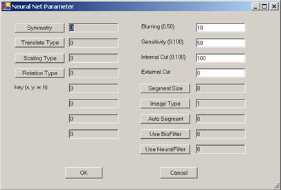
Figure 16.6 Neural Net Parameter.
The available NeuralNet filters are:
- 100x100 (Most Accurate)
- 90x90
- 80x80
- 70x70
- 60x60
- 50x50 (Least Accurate)
Let the speed of 100x100 filter be a base, then the overall speed for:
- 90x90 filter is 1 times faster;
- 80x80 filter is 1.6 times faster;
- 70x70 filter is 2.7 times faster;
- 60x60 filter is 5 times faster; and
- 50x50 filter is 10 times faster.
The NeuralNet Filter has many parameters. The following sections will explain these parameters.
16.6.1 Symmetry
Symmetry or Invariance means similarity under certain types of changes. For example, considering two images, one with a face in the middle and the other with the face moved to the edge; we say these two images are similar because of the face.
The symmetry defines "similar images". The Attrasoft ImageFinder supports five symmetry settings:
· No symmetry (0);
· Translation symmetry (3);
· Scaling symmetry (4);
· Rotation symmetry (5); and
· Rotation & Scaling symmetries (6).
The numbers are the codes in the batch file. Currently, Scaling symmetry and Oblique symmetry are the same.
A customized Attrasoft ImageFinder can implement any symmetry (or combination of symmetries), which can be described by mathematics. However, symmetries are computationally expensive.
Every symmetry setting has the Translation symmetry, except "No Symmetry". In addition, each of the above settings support:
· Intensity symmetry.
Symmetries are computationally expensive, meaning it will take a longer time to do the job. You should use them only when they are required.
To set the Symmetry, keep clicking the Symmetry button; the setting will switch from one to the next each time you click the button. The default setting in this version is Translation Symmetry.
For example, it seems that Stamp Recognition requires Translation and Rotation symmetries. But because the edges of a stamp can be detected easily, the stamp can be rotated and shifted to a fixed position where the horizontal side is longer than the vertical side. All you need to do is recognize a stamp or an upside-down stamp. Therefore, Stamp Recognition does not really require Translation and Rotation symmetries.
16.6.2 Translation Type
The Translation Type defines the accuracy of the Translation symmetry.
The Translation Type settings (and their codes) are:
· Most Accurate (0);
· Accurate (1); and
· Least Accurate (2).
To set the Translation Type, keep clicking the “T Type” button; the setting will switch from one to the next each time you click the button. The default setting is 0, the most accurate setting.
16.6.3 Scaling Type
The Scaling Type defines the accuracy of the Scaling symmetry.
The Scaling Type settings (and their codes) are:
· Least Accurate (0);
· Accurate (1);
· Accurate (2); and
· Most Accurate (3).
To set the Scaling Type, keep clicking the “T Type” button; the setting will switch from one to the next each time you click the button. The default setting is 0, the least accurate setting.
16.6.4 Rotation Type
The Rotation Type defines the accuracy of the Rotation symmetry.
The Rotation Type settings (and their codes) are:
· 360° rotation, least accurate (0);
· -5° to 5° rotation (1);
· -10° to 10° rotation (2);
· 360° rotation, accurate (3);
· 360° rotation, more accurate (4);
· 360° rotation, most accurate (5).
To set the Rotation Type, keep clicking the “Rotation Type” button; the setting will switch from one to the next each time you click the button. The default setting is 360° rotation, the least accurate setting (0).
16.6.5 Area of Interest (AOI)
The key is created by cropping out the AOI from an image. Figure 9.4 in chapter 9 shows an example.
16.6.6 Blurring
This is one of the most important search parameters and the first parameter you should adjust. Blurring compensates for minor image changes, which are not visible to human eyes. For example, if you use software to compress an image, to change the intensity of an image, or to translate, scale, or rotate an image, the image will be distorted a bit at the pixel level. You have to set “Blurring” to compensate for this.
To Summarize:
- When a search
yields no results, increase Blurring;
- When a search
yields too many results, decrease Blurring.
16.6.7 Sensitivity
The Sensitivity parameter ranges from 0 (least sensitive) to 100 (most sensitive).
- To search small segment(s), use high sensitivity search.
- To search large segment(s), use low sensitivity search.
- The higher this parameter is, the more results you will get.
16.6.8 Internal/External Weight Cut
You can set the "Internal Weight Cut" (Internal Cut) or "External Weight Cut" (External Cut) to list only those retrieved images with scores or weights greater than a certain value (called Threshold).
It is better to give no answer than a wrong answer. Assume you are searching images and all similar images have weights ranging from 1,000 to 10,000. It is possible that some other images pop up with weights ranging from 10 to 100. To eliminate these images, you can set the “External Weight Cut” to 1,000.
The Internal Cut plays a similar role as the External Cut. There are two differences between these two cuts:
· The Internal Cut ranges from 0 to 99; the External Cut can be any number;
· The Internal Cut stops the images from coming out, whereas the External Cut can bring the eliminated images back if you set the External Cut to 0. You might need to see the eliminated images sometimes for the purpose of adjusting the parameters.
To Summarize:
·
Set the
“Internal Cut” or “External Cut” to eliminate errors.
16.6.9 Segment Size
To search large segments, use setting 0.
To search small segments, use setting 1.
For example:
- If a sample segment is one quarter of the sample image, it is a large segment.
- If the segment is 1/20 of the sample image, it is a small segment.
Currently, "S Segment" only supports Translation symmetry. If you need Rotation or/and Scaling symmetry, please use "L Segment".
16.6.10 Image Type
There are BW and Color images. For each of them, there are “sum-search”, “maximum-search”, and “average-search”. This generates 6 image types:
- BW Sum
- BW Max
- BW Avg
- Color Sum
- Color Max
- Color Avg
"BW Sum” is like an integration of function f (x).
"BW Max” is like a maximum value of f (x); and
"BW Avg” is the average of the above two.
"Color Sum” is like an integration of function f (x).
"Color Max” is like a maximum value of f (x); and
"Color Avg” is the average of the above two.
To set the image type, keep clicking the Image Type button; the setting will switch from one to the next each time you click the Image Type button.
16.6.11 Auto Segment
The training segment can be specified in two ways:
Manual Specification
Automatic Specification
The default is Manual Specification. In this
setting, the segment will be specified by the four text boxes (x, y, w, h), as
we discussed earlier.
If you do not want to pick up a training segment, then let the ImageFinder pick up the segment for you by using the Automatic Specification. This parameter has several settings:
NO Auto Segment
Very Large Segment
Very Large Segment
Large Segment
Large Segment
Medium Segment
Medium Segment
16.6.12 Summary
The NeuralNet filter is hard to use because it has so many parameters. Not all parameters are equal. We divide the parameters into two groups. The beginners should use only parameters in the first group. Note that:
- The most important parameters for Training are Image Processing, AOI, Symmetry, and Segment Cut (in the Reduction Filter).
- The most important parameters for Matching are Blurring, and Sensitivity.
In a typical search, you will
set these parameters and leave other parameters with the default values.
These are the 7 parameters you should focus on first:
Training (3 parameters):
- Segment: selecting “Large AutoSeg 3” so the ImageFinder will select a training segment for you at the beginning.
- Segment Cut (in the Reduction Filter)
Matching (4 parameters):
- Sensitivity
- Blurring
- External Weight Cut
- Internal Weight Cut
Ignore the rest of the parameters at the beginning.
17. Application Developers
This chapter answers some common questions raised by image recognition solution developers.
17.1 Application Structure
An image recognition application is roughly divided into:
Level 5: User
Interface;
Level 4: Data Management;
Level 3: Image-Matching Layer;
Level 2: Scanner, Camera, and their drivers;
Level 1: PC with Windows.
Attrasoft provides programming tools for the image matching layer through customization.
17.2 Available Products
The ImageFinder
family has several products:
ImageFinder for Windows is off-the-shelf application software that enables a quick testing of Image Recognition ideas.
VideoFinder for Windows is off-the-shelf application software that enables a quick testing of Video Recognition ideas.
TransApplet is .Net Class Library that enables addition of Image/Video Recognition capability to products & services.
AttraSeek is off-the-shelf web application software (http://attraseek.com).
17.3 Development Procedure
The
Image Recognition Solution Development Procedure is:
(1)
Set up the system (you will do that).
(2)
Collect the data (you will do that).
(3)
Preliminary Assessment via our off-the-shelf software, the ImageFinder.
You should get Identification Rates ranging from 60%
to 89%. The best rate, one of our customers (without any customization) was
able to obtain, was an 89% Identification Rate.
Note: The off-the-shelf ImageFinder has many
open parameters for users to adjust, which is the reason customers are only
able to achieve Identification Rates ranging from 60% to 89%.
(4) Feasibility Project via Customized
Stand-alone Software.
·
The ImageFinder itself has 3,000+ internal parameters to which
users have no access.
·
Customization is the process of adjusting these 3,000+ internal
parameters for your specific image type; this is where the high degree of
accuracy for your specific image type is obtained.
·
ATTRASOFT will develop a stand-alone software, which will address the
special needs / requirements of your application. This will allow you to show
your upper management the practicality of a larger project.
(5)
Programming Library in .Net.
Attrasoft will provide you with an API and develop a
.Net class library for your application(s).
(6)
System Integration to your Production Line.
Attrasoft will provide Support to your system
integration.
(7)
Licensing & Annual Maintenance.
18. Selected Reference Manual
18.1 Signature Menu
Signature/1:1 First Signature
Use the “Signature/1:1 First Signature” menu item to compute the signature of the specified key image. This menu item has no direct application in the software; it merely shows users what a signature looks like.
Signature/1:1 Second Signature
Use the “Signature/1:1 Second Signature” menu item to compute the signature of the image on the middle picture box. This menu item has no direct application in the software; it merely shows users what a signature looks like.
Signature/1:N Signature (.\data\a1.txt)
Use the menu item “Signature/1:N Signature (.\data\a1.txt)” to compute the signatures specified in the search source and save the signature in a1.txt. This file will be used for 1:N Matching and N:N Matching.
Signature/M:N Signature (.\data\a2.txt)
Use the menu item “Signature/M:N Signature (.\data\a2.txt)” to compute the signatures specified in the search source and save the signature in a2.txt. This file will be used for N:N Matching.
Signature/N Signature (a3.txt)
Use the menu item “Signature/N Signature (a1.txt)” to compute the signatures specified in the search source and save the signature in a3.txt. This file will be used for 1:N Matching and N:N Matching.
18.1.1 Variation Signatures
The “Signature/Variation Signatures” menu item provides a list a menu items to compute signatures. The net result is that an image will have multiple image signatures.
The “Signature/Variation Image” menu item will compute various variations of images from the key image and will deposit these images into “.\tmp\” folder. To use this menu item, you must first select a key image. This allows a user to see what the variations are.
To get signatures for images in a folder in your computer:
1. Select a folder;
2. Click one of the menu items below.
Signatures/Scale (100, 90, 80, …)
This menu item generates 7 image signatures:
100%, 90%, 80%, 70%, 60%, 50%, 40%.
Here 90% is an image that has 5% border region removed.
Signatures/Rotation (90, 180, 270)
This menu item generates 4 image signatures:
0, 90, 180, 270.
Here 90 is an image that has a 90 degree rotation.
Signatures/Flip (X, Y, XY)
This menu item generates 4 image signatures:
0, X, Y, XY.
Here X is an image that has flipped around x axis.
Signature/Flip Rotation (16 variations)
This menu item generates 16 image signatures:
{0, 90, 180, 270} ^ {0, X, Y, XY}.
Here (90, X) is an image that has 90 degree rotation and flipped around x axis.
Signature/Stretch (4 variations)
This menu item generates 5 image signatures:
(0,0), (120%, 100%), (80%, 100%), (100%, 120%), (100%, 80%).
Here (120%, 100%) are stretch percentages along the x and y directions.
Signature/Resize
This menu item generates 5 image signatures:
100, 150, 200, 300, 400.
Here 150 increases the image size by 50% in terms of pixel counts in each direction.
18.2 Whole Image
Whole Image/1:1 Matching
Use the “Whole Image/1:1 Matching” menu item to make a 1:1 matching.
Whole Image/1:N Matching
Use the “Whole Image/1:N Matching” menu item to make a 1:N matching.
18.3 Analysis
“Analysis/Open results (b1.txt)” Menu Item
Use the “Analysis/Open results
(b1.txt)” menu item to open b1.txt, which is the file containing the last
matching result in text format.
“Analysis /Html Without Images” Menu Item
Use the “Analysis /Html Without
Images” menu item to open b1.htm, which is the file containing the last
matching result in html format.
“Analysis /Html With Images” Menu Item
Use the “Analysis /Html With
Images” menu item to open b1.html, which is the file containing the last
matching result in html format, with both input images and output images
displayed in the web page.
“Analysis /Check” Menu Item
Use the “Analysis /Check” menu
item to compute the number of matches in the output file, b1.txt, are expected
from b1_matchlist.txt.
18.4 Binary Search
Binary Search/Create sort1.txt from a1.txt
Use the “Binary Search/Create sort1.txt from a1.txt” menu item to create binary search file.
Binary Search/1:N Search (key vs. sort1.txt)
Binary Search/1:N Search (10%)
Binary Search/1:N Search (5%)
Binary Search/1:N Search (3%)
Binary Search/1:N Search (1%)
Use the one of the menu items to make 1:N match.
18.5 Library
18.5.1 Maintenance
Library/Maintenance/Create lib1.txt from a1.txt
Use the “Library/Maintenance/Create lib1.txt from a1.txt” menu item to create library file lib1.txt.
Library/Maintenance/Load lib1.txt
Use the “Library/Maintenance/Load lib1.txt” menu item to load library file lib1.txt.
“Library/Maintenance/Print Library” Menu Item
Use the “Library/Maintenance/Print Library” menu item to print the library to the text window.
“Library/Maintenance/Clear Library” Menu Item
Use the “Library/Maintenance/Print Library” menu item to clear the current library.
“Library/Maintenance/Backup (lib1_bk.txt)” Menu Item
Use the “Library/Maintenance/Backup (lib1_bk.txt)” menu item to create a backup copy of the currently loaded library to lib1_bk.txt.
“Library/Maintenance/Save
lib1.txt, lib2.txt to lib3.txt” Menu Item
Use the “Library/Maintenance/Save lib1.txt, lib2.txt to lib3.txt” menu item to create a combination of the two library files, lib1.txt and lib2.txt, into a new library file, lib3.txt. To use this file, save it to lib1.txt, or lib2.txt, and load.
“Library/Maintenance/Add (Key)” Menu Item
Use the “Library/Maintenance/Add (Key)” menu item to add a signature to the loaded library. The inserted signature is computed from the key image.
“Library/Maintenance/Delete (Key)” Menu Item
Use the “Library/Maintenance/Delete (Key)” menu item to delete a signature from the loaded library. The deleted signature is computed from the key image.
“Library/Maintenance/Replace (Key)” Menu Item
Use the “Library/Maintenance/Replace (Key)” menu item to replace a signature in the loaded library. The replaced signature is computed from the key image.
18.5.2 Matching
Library/1:N Matching (Key vs. lib1.txt)
Use the “Library/1:N Matching (Key vs. lib1.txt)” menu item make a 1:N match.
18.6 Training
Whole/Training/Training Without Saving Menu Item
Use the “Whole/Training/Training Without Saving” menu item to train the ImageFinder.
18.7 Sub Images
Sub Image/1:1 Matching Menu Item
Use the “Sub Image/1:1 Matching” menu item to make a 1:1 Matching.
Sub Image/1:N Matching Menu Item
Use the “Sub Image/1:N Matching” menu item to make a 1:1 Matching.
Sub Image/Fast 1:1
Use “Sub Image/Fast 1:1” to make a 1:1
Matching.
Sub Image/Fast 1:N (Same size)
Use
“Sub Image/Fast 1:N (Same size)” to make a 1:N Matching; it will
search through all images in a folder for the specified cropped image. This
command is faster than “Sub Image/1:N (Different size)”, but
it requires all images in the search folder to have the same pixel size.
Sub Image/Fast 1:N (Different size)
Use
“Sub Image/Fast 1:N (Different size)” to make a 1:N Matching; it
will search through all images in a folder for the specified cropped image.
This command is slower than “Sub Image/1:N (Same size)”, but it
does not requires all images in the
search folder to have the same pixel size.